  density pred  size surv propsurv
1      10   no   big    9      0.9
2      10   no   big   10      1.0
3      10   no   big    7      0.7
4      10   no   big   10      1.0
5      10   no small    9      0.9
6      10   no small    9      0.9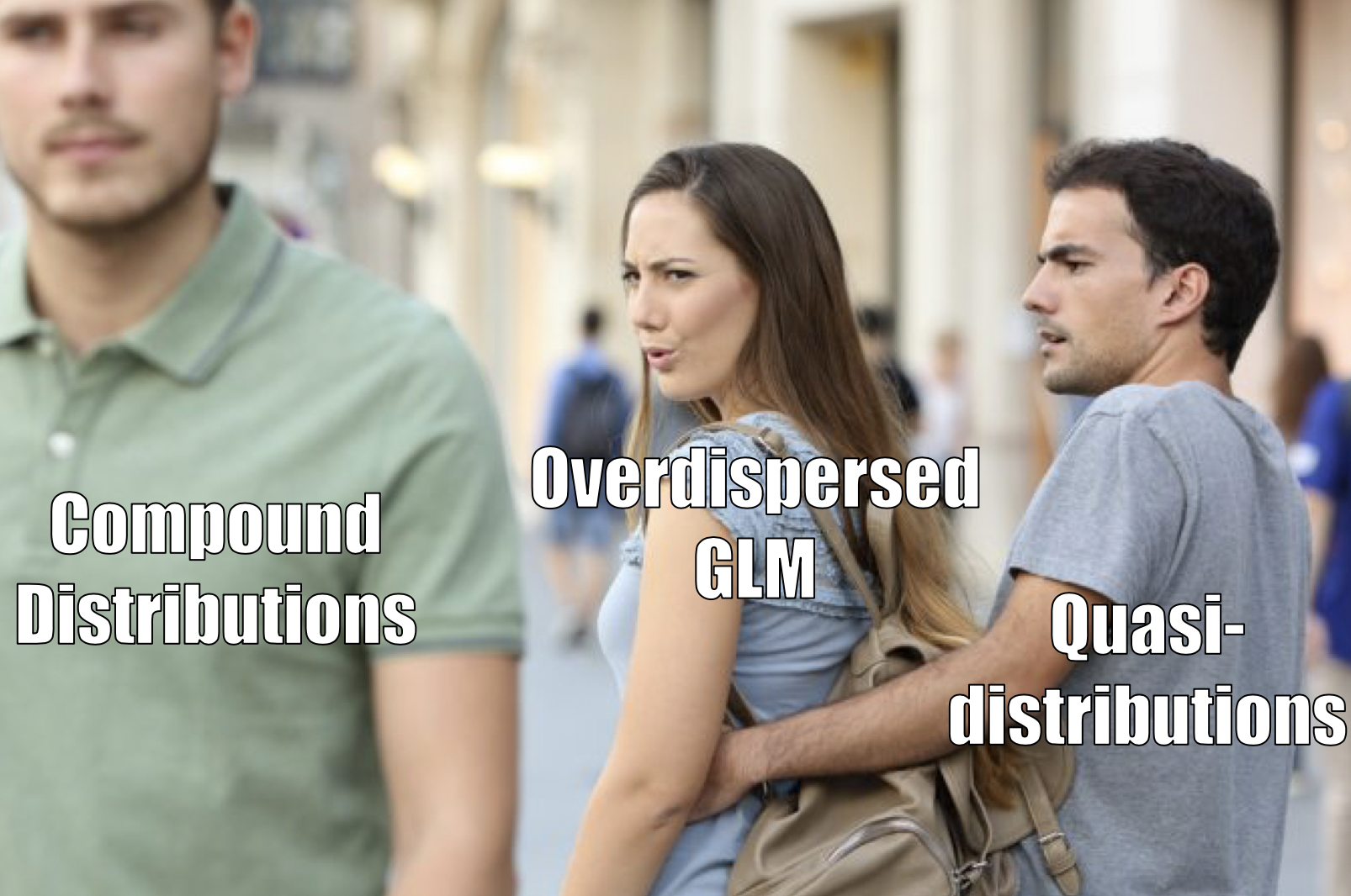
Reed frogs
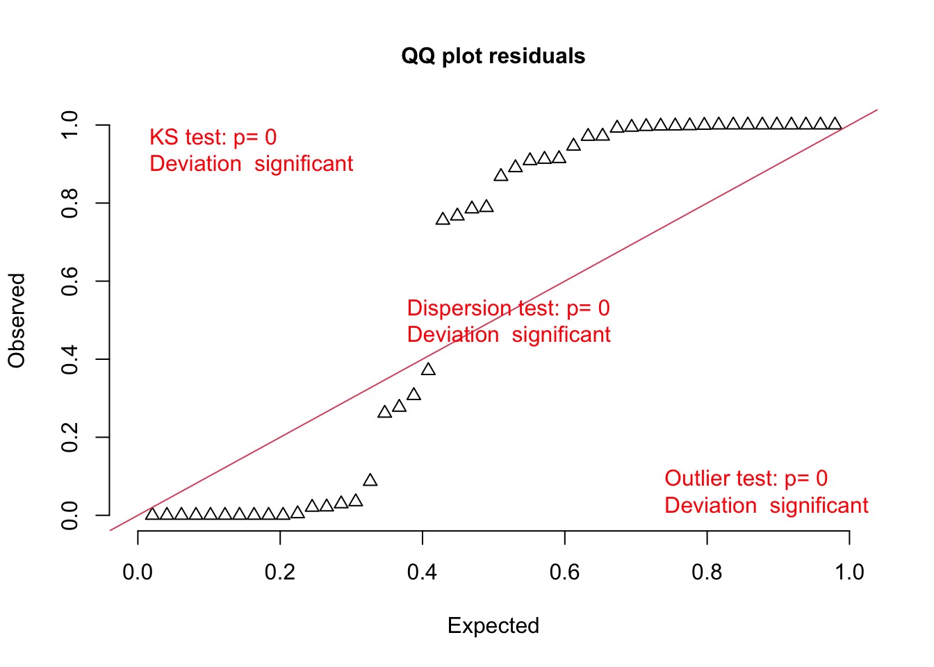
But those QQ plots…
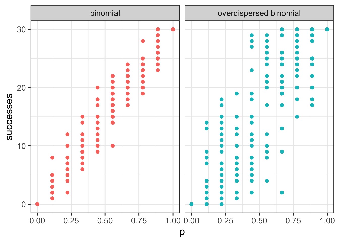
Overdispersed Binomial
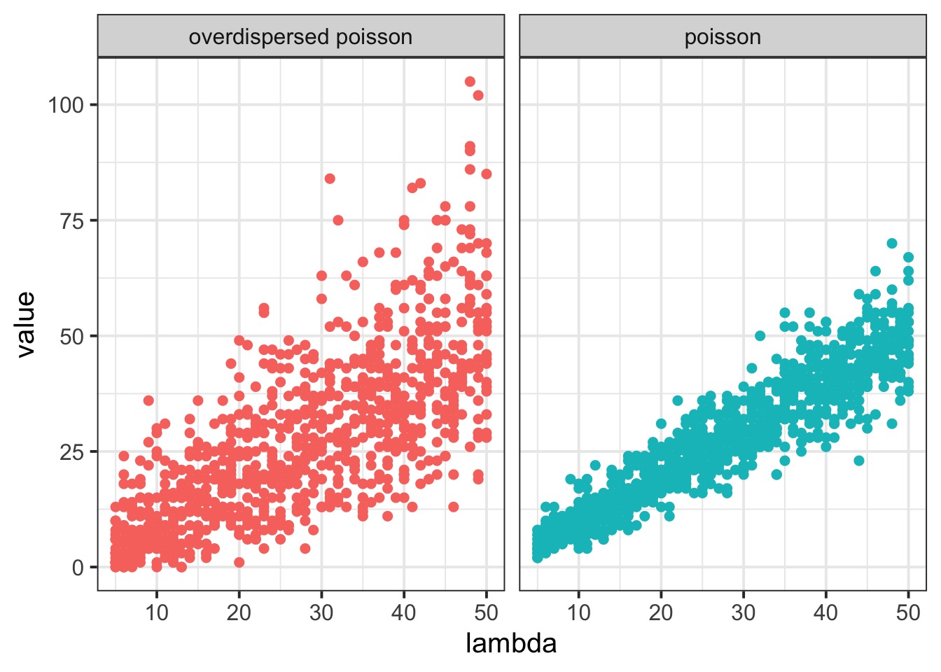
Overdispersed Poisson
Mixture-based solutions
We can mix distributions in two ways
First, we can apply a scaling correction - a Quasi-distribution
OR, we can mix together two distributions into one!
Let’s Cook with Flame: Pure Mixture Distributions

Consider…
\(X \sim Bin(n,p)\)
\(p\sim Beta(\alpha,\beta)\)
with \(\alpha = p \theta\) and \(\beta = (1-p) \theta\)
or
\(p\sim BetaBin(n, \hat{p},\theta)\)
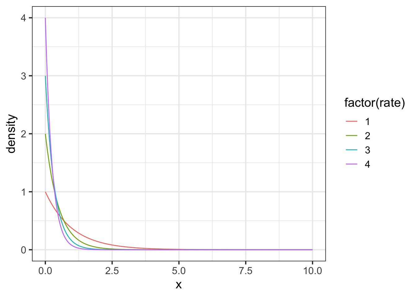
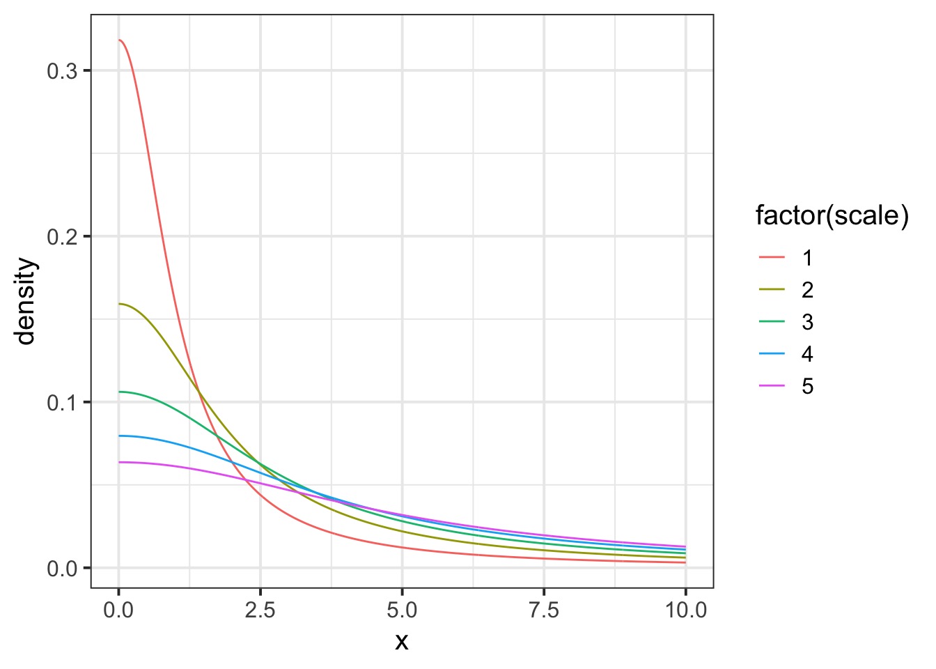
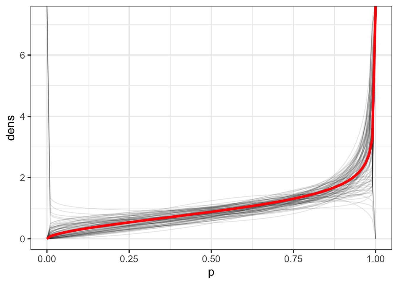
The Beta
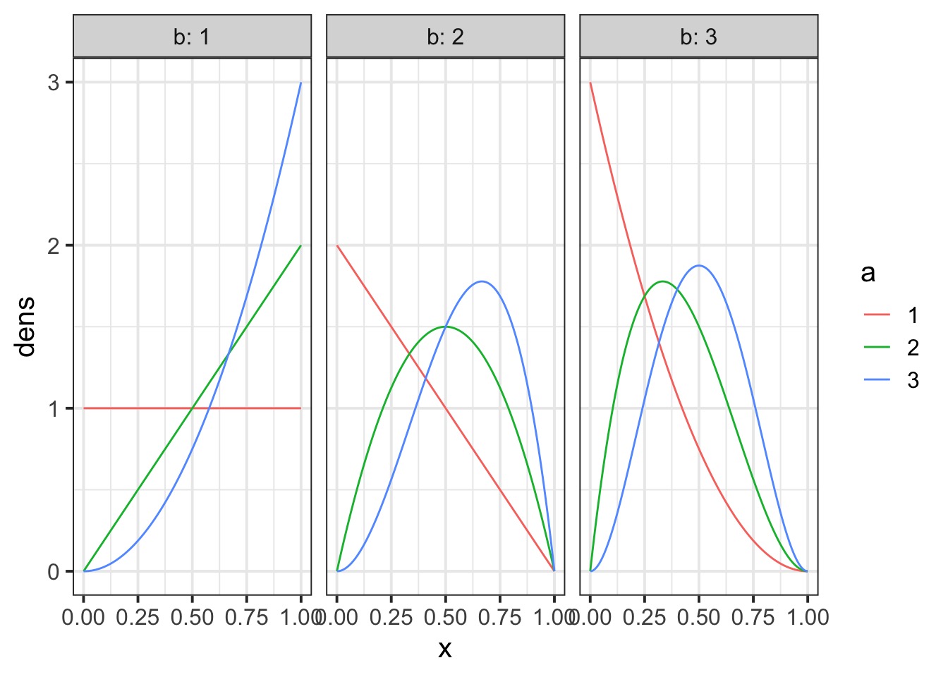
How does the beta binomial change things?

How does the beta binomial change things?

How does the beta binomial change things?

How does the beta binomial change things?

An Exponential Prior?
Or An Cauchy Prior?
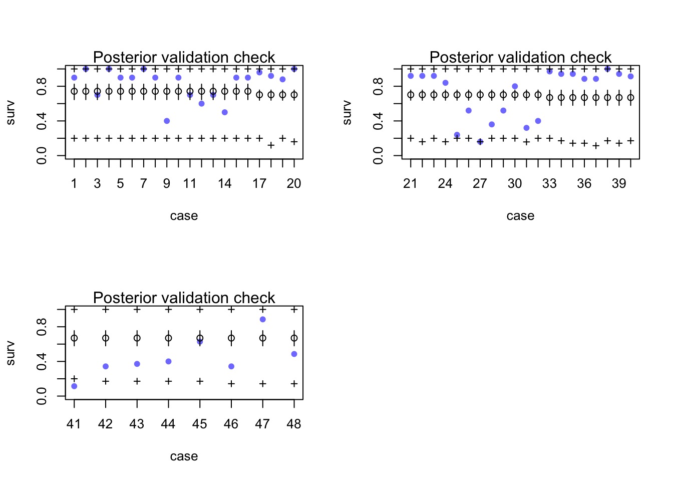
Let’s look at an estimate!
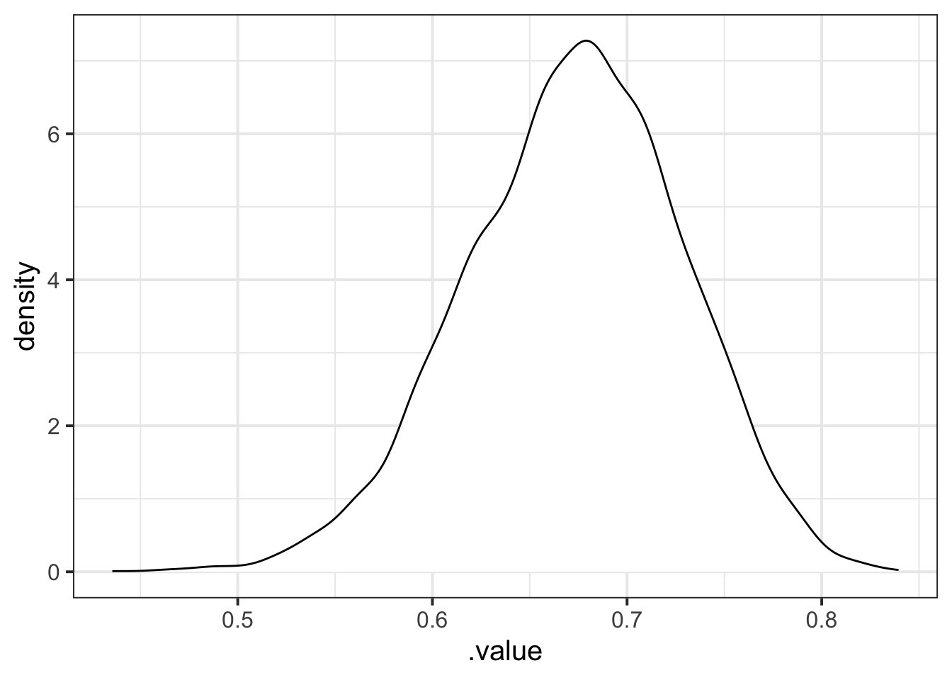
How does Overdispersion Affect this?
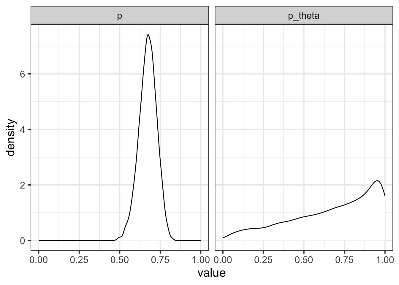
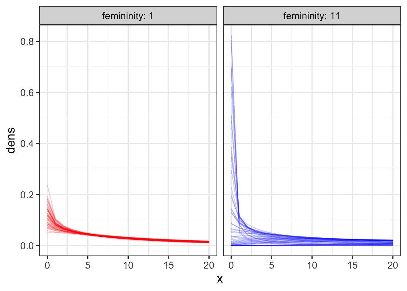
Variability in Overdispersion by Draw
Did this solve our overdispersion problem?
Results
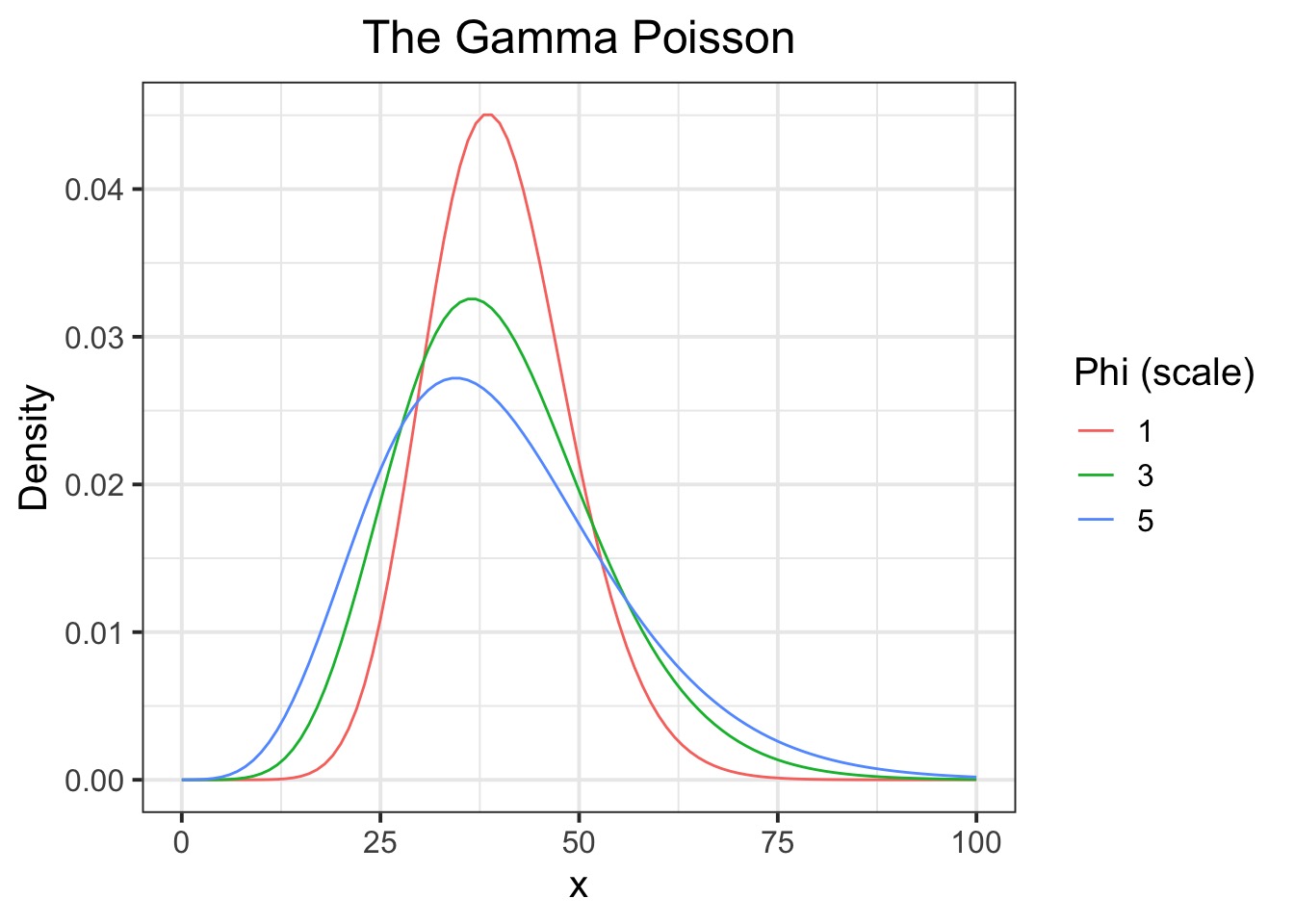
Hurricanes and Gamma Poisson
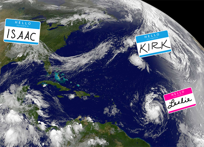
Discover Magazine
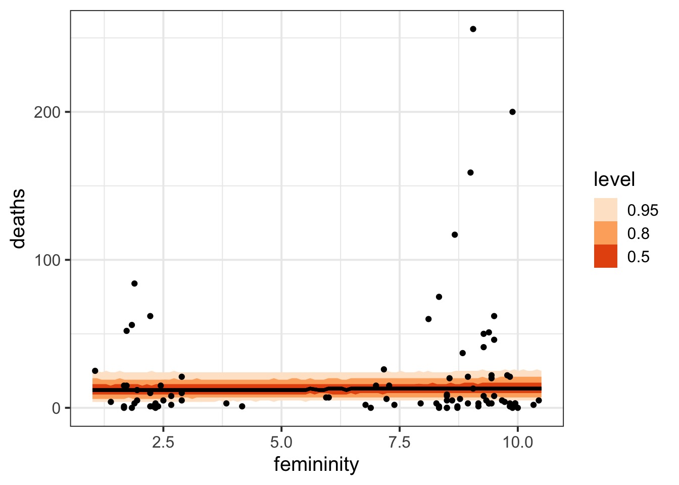
Overdispersed hurricanes
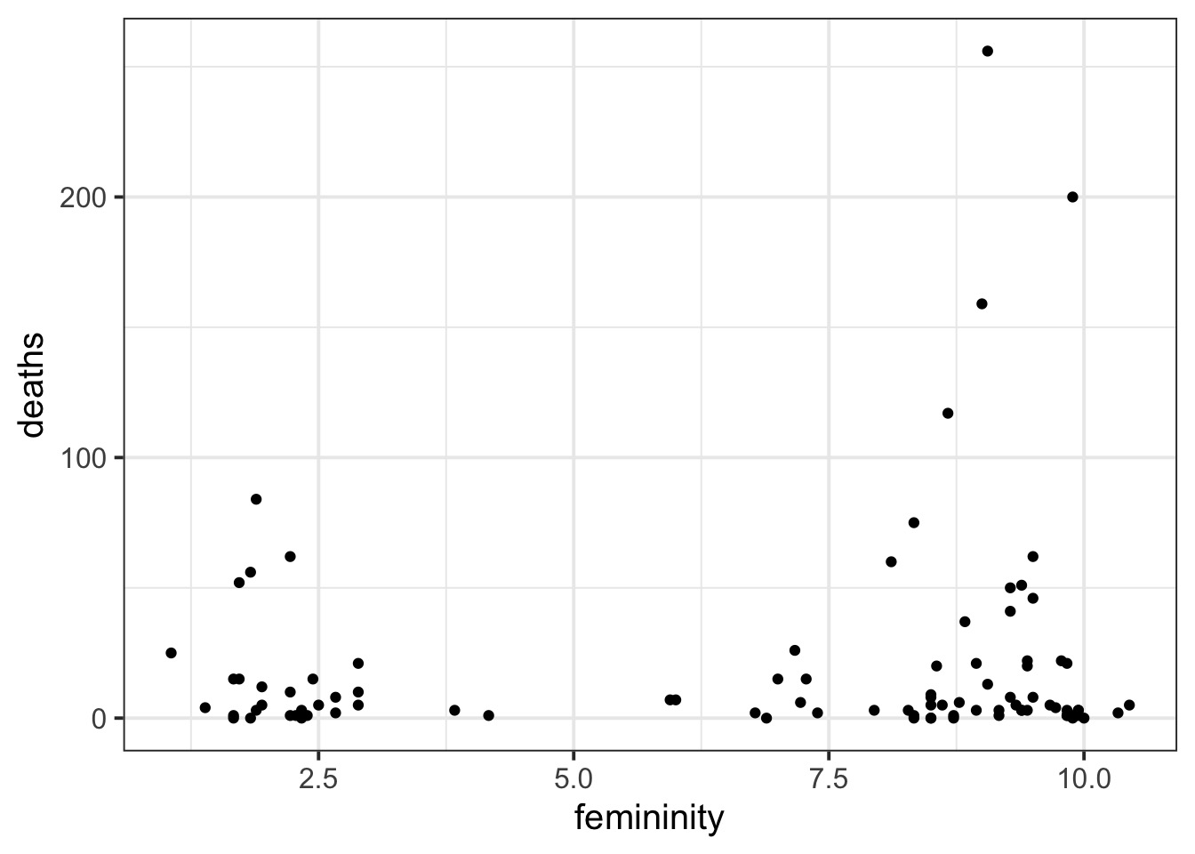
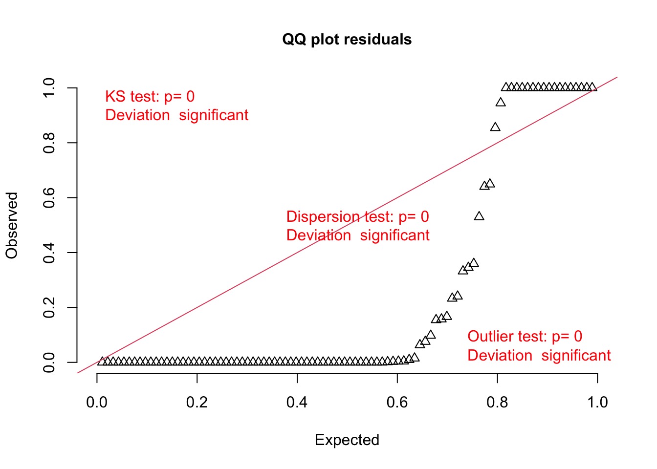
Poisson?
The Distribution (mean of 40)
Let’s look at the residuals
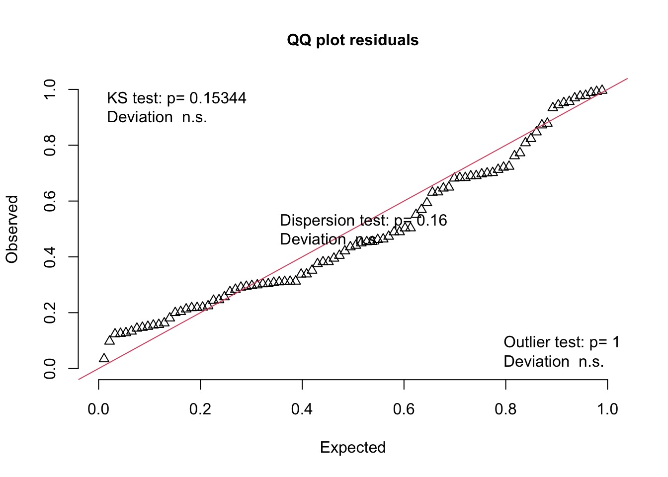
Did it Work?
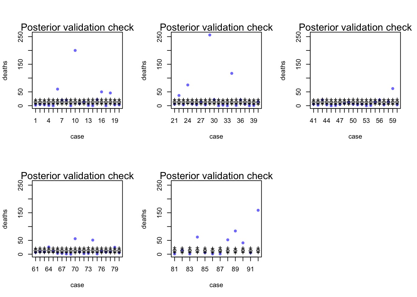
Evaluating Posterior Predictions
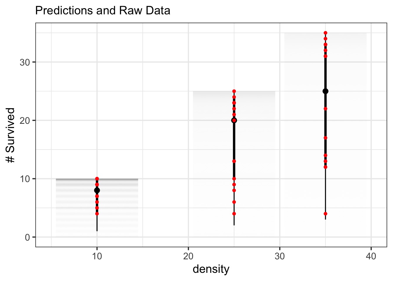
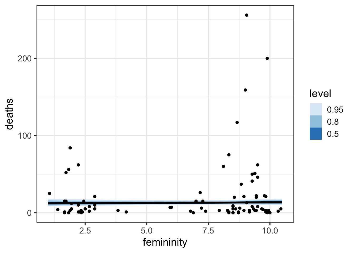
Did it Predict Well?
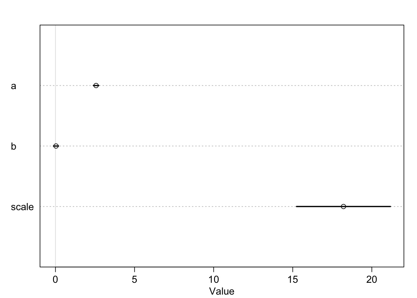
Wait, Those Coefs…
Well, What did the Predictions Say