Bayesian Models with Multiple Predictors

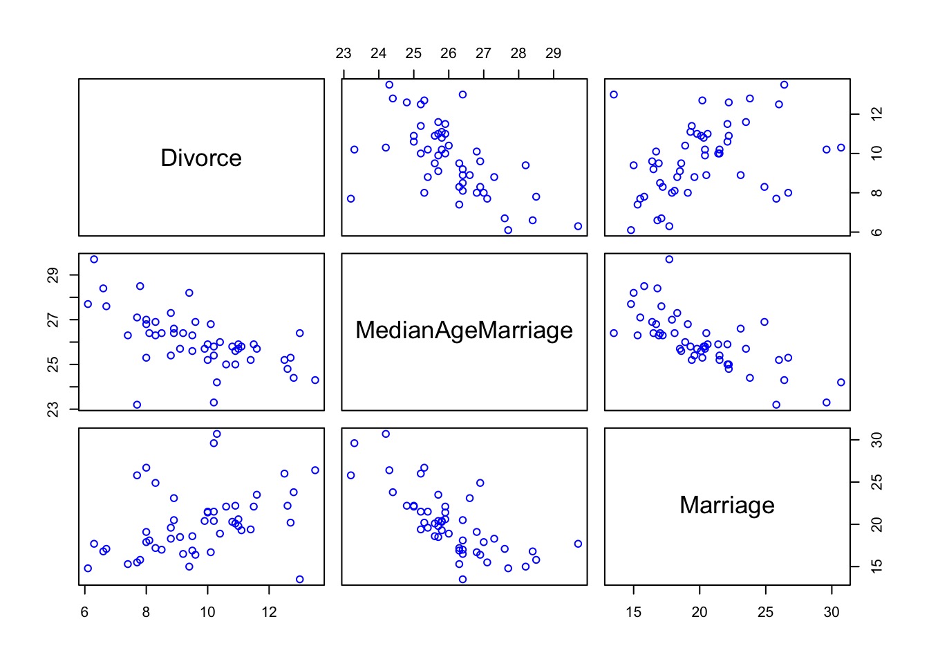
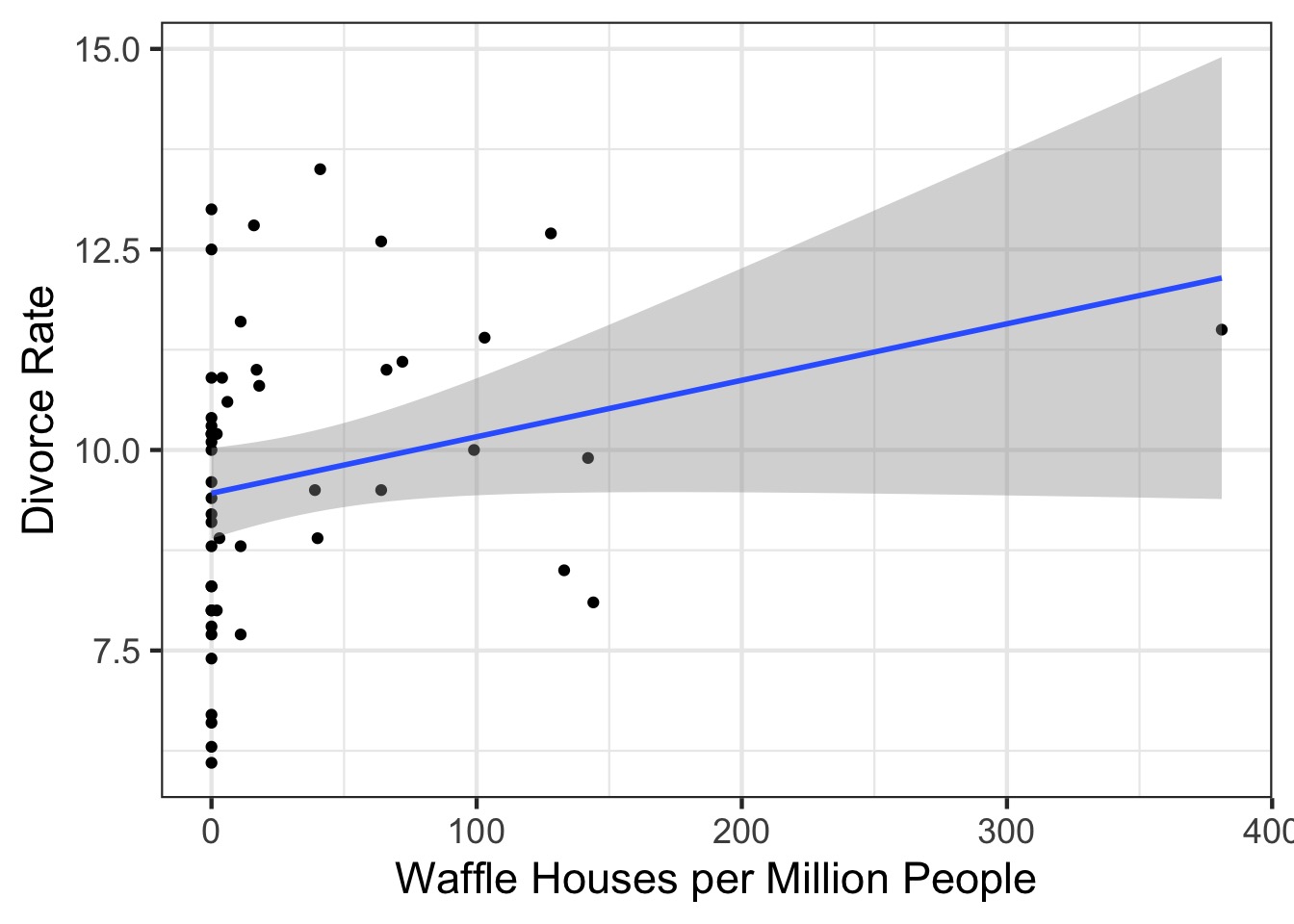
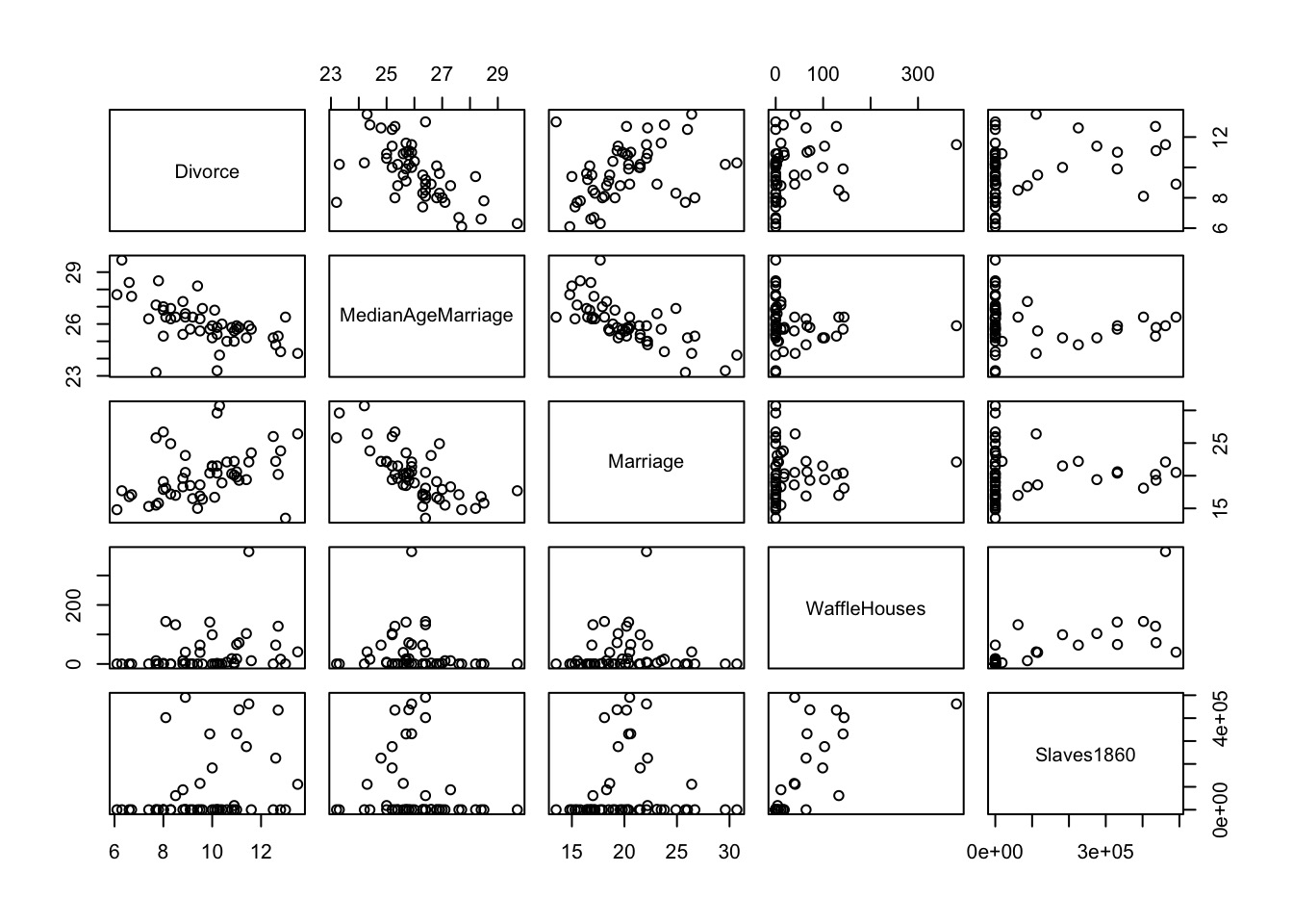
Waffle House: Does it Lead to Perdition?

So many possibilities

Today’s Outline

Multiple Predictors in a Bayesian Framework
- How multiple predictors tease apart spurious and masked relationships
Evaluating a Model with Multiple Predictors
Testing Mediation
Categorical Variables

Why use multiple predictors

Controlling for confounds
- Disentangle spurious relationships
- Reveal masked relationships
Dealing with multiple causation
Interactions (soon)

Why NOT use multiple predictors

Multicollinearity
- But can aggregate variables
Overfitting
- But see model selection
Loss of precision in estimates
Interpretability

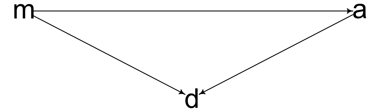
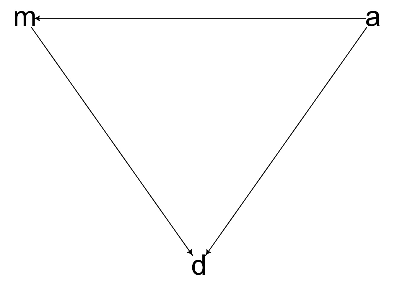
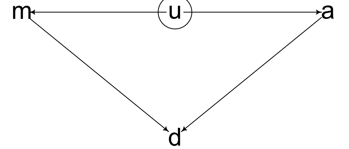
DAG Before You Model

Which of these is your model?

Should we Standardize?

Standardization can aid in fitting.
- No scaling issues
- Faster convergence
- Reduces collinearity of derived predictors (nonlinear terms)
Standardization X and/or Y can aid in choosing priors
- Centering moves intercept to 0 on X and/or Y axis
- Dividing by SD means we can think in terms of standard normal for slopes and intercepts
Interpretation
- For linear models, coefficients are standardized correlation coefficients
- Can back-transform Y by multiplying by sd and adding mean

Let’s Standardize Divorce

WaffleDivorce <- WaffleDivorce |>
  mutate(D = (Divorce - mean(Divorce))/sd(Divorce),
         A = (MedianAgeMarriage - mean(MedianAgeMarriage))/sd(MedianAgeMarriage),
         M = (Marriage - mean(Marriage))/sd(Marriage))

Or use standardize() or write a function

How to Build a Model with Multiple Predictors

Likelihood:
\(y_i \sim Normal(\mu_i, \sigma)\)

Data Generating Process
\(\mu_i = \alpha + \beta_1 x1_i + \beta_2 x2_i + ...\)

Prior:
\(\alpha \sim Normal(0, 0.5)\)
\(\beta_j \sim Normal(0, 0.5)\) prior for each
\(\sigma \sim Exp(1)\)

Our Model

Likelihood:
\(D_i \sim Normal(\mu_i, \sigma)\)

Data Generating Process
\(\mu_i = \alpha + \beta_m M_i + \beta_a A_i\)

Prior:
\(\alpha \sim Normal(0, 0.5)\) because standardized
\(\beta_m \sim Normal(0, 0.5)\) because standardized
\(\beta_a \sim Normal(0, 0.5)\) because standardized
\(\sigma \sim Exp(1)\) because standardized

Our Model

mod <- alist(
  #likelihood
  D ~ dnorm(mu, sigma),
  
  #data generating process
  mu <- a + bM*M + bA * A,
  
  # Priors
  a ~ dnorm(0, 0.5),
  bM ~ dnorm(0, 0.5),
  bA ~ dnorm(0, 0.5),
  sigma ~ dunif(0,10)
)

fit <- quap(mod, data=WaffleDivorce)

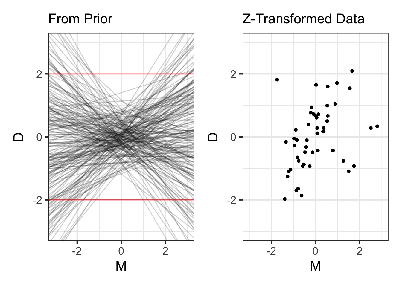
Were Our Priors Reasonable?

Prior for Marriage Age N(0,0.5)

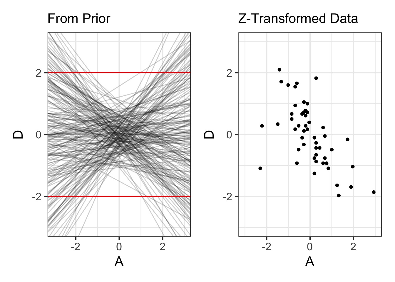
Prior and Plot

prior_divorce <- extract.prior(fit, n = 200) |> 
  as_tibble()

p1 <- ggplot(data = prior_divorce) +
  geom_abline(aes(slope = bA, intercept = a), alpha = 0.2) +
  xlim(c(-3,3)) + ylim(c(-3,3))  +
  geom_hline(yintercept = c(-2,2), color = "red") +
  labs(y = "D", x = "A", subtitle = "From Prior")


d1 <- ggplot(data = WaffleDivorce) +
  geom_point(aes(x = A, y = D)) +
    xlim(c(-3,3)) + ylim(c(-3,3))  +
  labs(subtitle = "Z-Transformed Data")


p1 + d1

Were Our Priors Reasonable?

Prior for Marriage Rate N(0, 0.5)

Results: We Only Need Median Age

What does a Multiple Regression Coefficient Mean?

What is the predictive value of one variable once all others have been accounted for?
We want a coefficient that explains the unique contribution of a predictor
What is the effect of x1 on y after we take out the effect of x2 on x1?

Today’s Outline

Multiple Predictors in a Bayesian Framework
- How multiple predictors tease apart spurious and masked relationships
Evaluating a Model with Multiple Predictors
Testing Mediation
Categorical Variables

How to Understand Posteriors

pairs(fit)

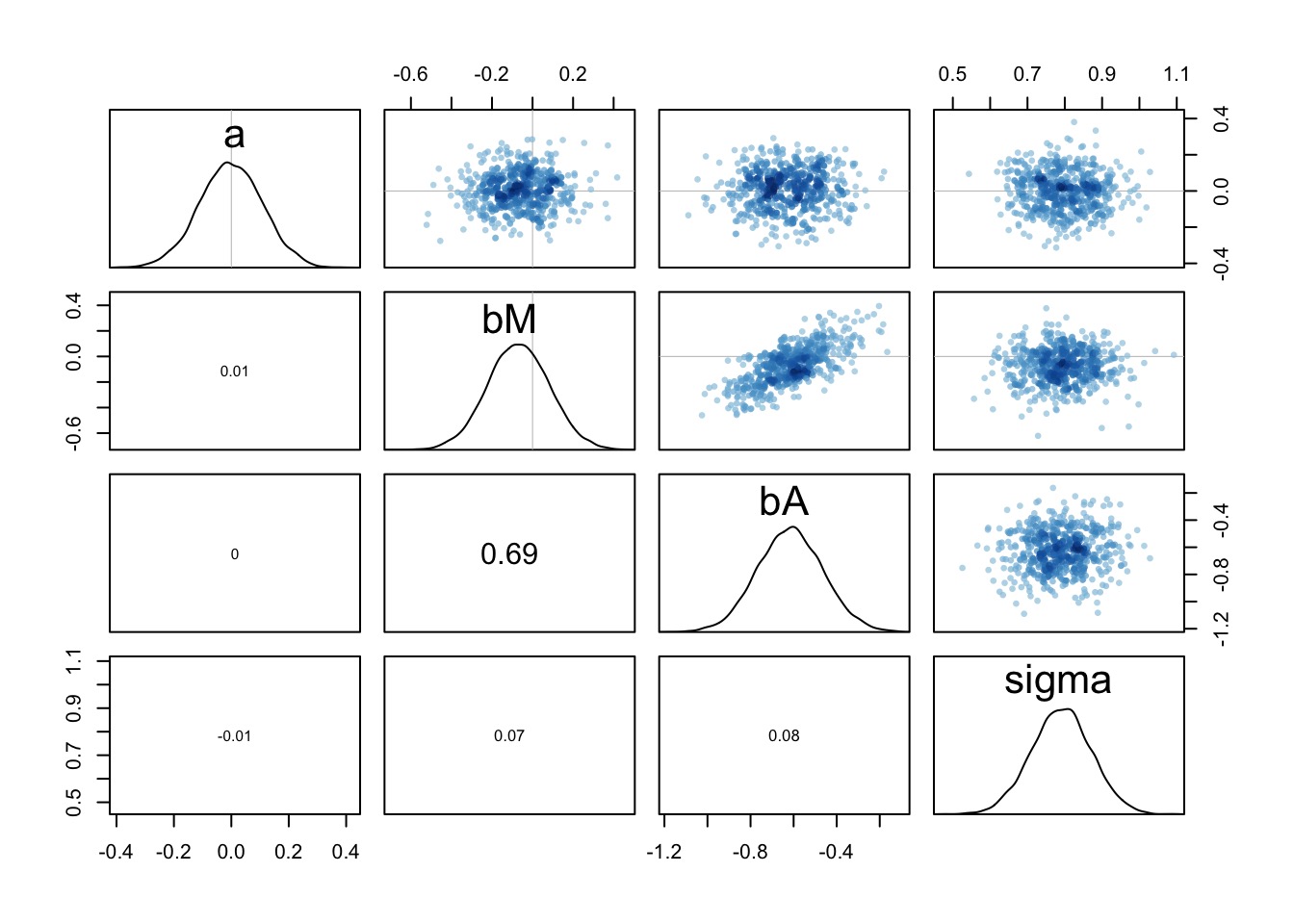
Note correlation between bM and bA - when one is high the other is as well, but see scale

How to Understand Posteriors

Predictor-residual plots
- What if you remove the effect of other predictors?
Counterfactual plots
- What if something else had happened?
Posterior Predictions
- How close are model predictions to the data

Predictor-Residual Plots

The cr.plots from the car package
- Component-residual
Take the residual of a predictor, assess it’s predictive power

Steps to Make Predictor-Residual Plots

Compute predictor 1 ~ all other predictors
Take residual of predictor 1
Regress predictor 1 on response

PR Model Part 1

m_mod <- alist(
  #model
  M ~ dnorm(mu, sigma),
  mu <- a + b*A,
  
  #priors
  a ~ dnorm(0,10),
  b ~ dnorm(0,10),
  sigma ~ dunif(0,10)
  )

m_fit <- quap(m_mod, data=WaffleDivorce)

PR Model Part 2

WaffleDivorce <- WaffleDivorce %>%
  mutate(Marriage_resid = M - 
           (coef(m_fit)[1] + coef(m_fit)[2]*A)
)

The Predictor-Residual Plot

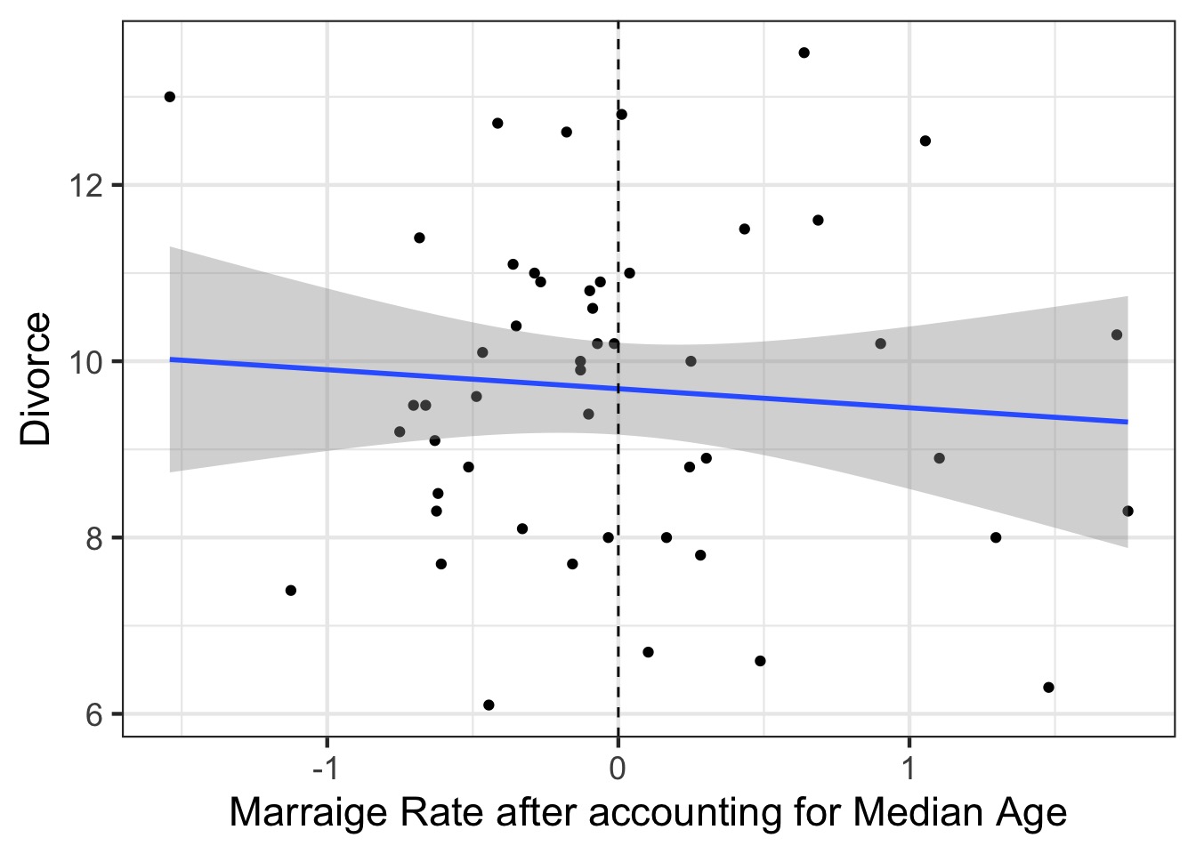
What have we learned after accounting for median age?

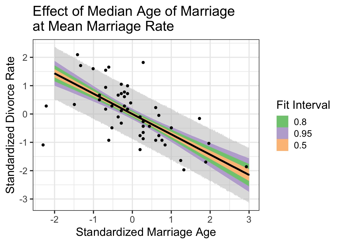
Counterfactual Plots

Counterfactual: A conditional statement of “if this, then …”
Powerful way of assessing models - “If we had seen Marriage Rate as x, then the effect of Median age on divorce rate would be…”
Shows model implied predictions, often at levels nor observed

But - WHICH if?

Estimate effect of Age and Rate controlling for one another

Estimate total, direct, & indirect effect of Age on Divorce

(This is Structural Equation Modeling)

Counterfactual Plots: Code

Effect of Age on Divorce holding Rate at it’s Mean

library(tidybayes)
library(tidybayes.rethinking)

# fit interval
cf_fit <- tidyr::crossing(A = seq(-2,3, .01),
                          M = 0) |>
  linpred_draws(m_fit, newdata = _)

# prediction interval
cf_pred <- tidyr::crossing(A = seq(-2,3, .01),
                          M = 0) |>
  predicted_draws(m_fit, newdata = _)

What do we learn about the effects of Median Marriage Age Alone?

Today’s Outline

Multiple Predictors in a Bayesian Framework
- How multiple predictors tease apart spurious and masked relationships
Evaluating a Model with Multiple Predictors
Testing Mediation
Categorical Variables

What if this was right?

Mediation

The effect of one variable has a direct and indirect effect
The indirect effect is mediated through another variable.
Multiple types of mediation
- Full mediation (i.e., no direct effect)
- Partial mediation (i.e., a direct and indirect effect)
- Unmediated relationship (direct effect only)
We can look at strength of indirect and direct effects to differentiate
- Or we can use model selection
- Adding indirect effects also allows tests of causal independence

Our New Model

Likelihoods:
\(D_i \sim Normal(\mu_{di}, \sigma_d)\)
\(M_i \sim Normal(\mu_{mi}, \sigma_m)\)

Data Generating Processes
\(\mu_{di} = \alpha_d + \beta_m M_i + \beta_a A_i\)
\(\mu_{mi} = \alpha_m + \beta_{ma} A_i\)

Prior:
\(\alpha_d \sim Normal(0, 0.5)\)
\(\alpha_m \sim Normal(0, 0.5)\)
\(\beta_m \sim Normal(0, 0.5)\)
\(\beta_a \sim Normal(0, 0.5)\)
\(\beta_{ma} \sim Normal(0, 0.5)\)
\(\sigma_d \sim Exp(1)\)
\(\sigma_m \sim Exp(1)\)

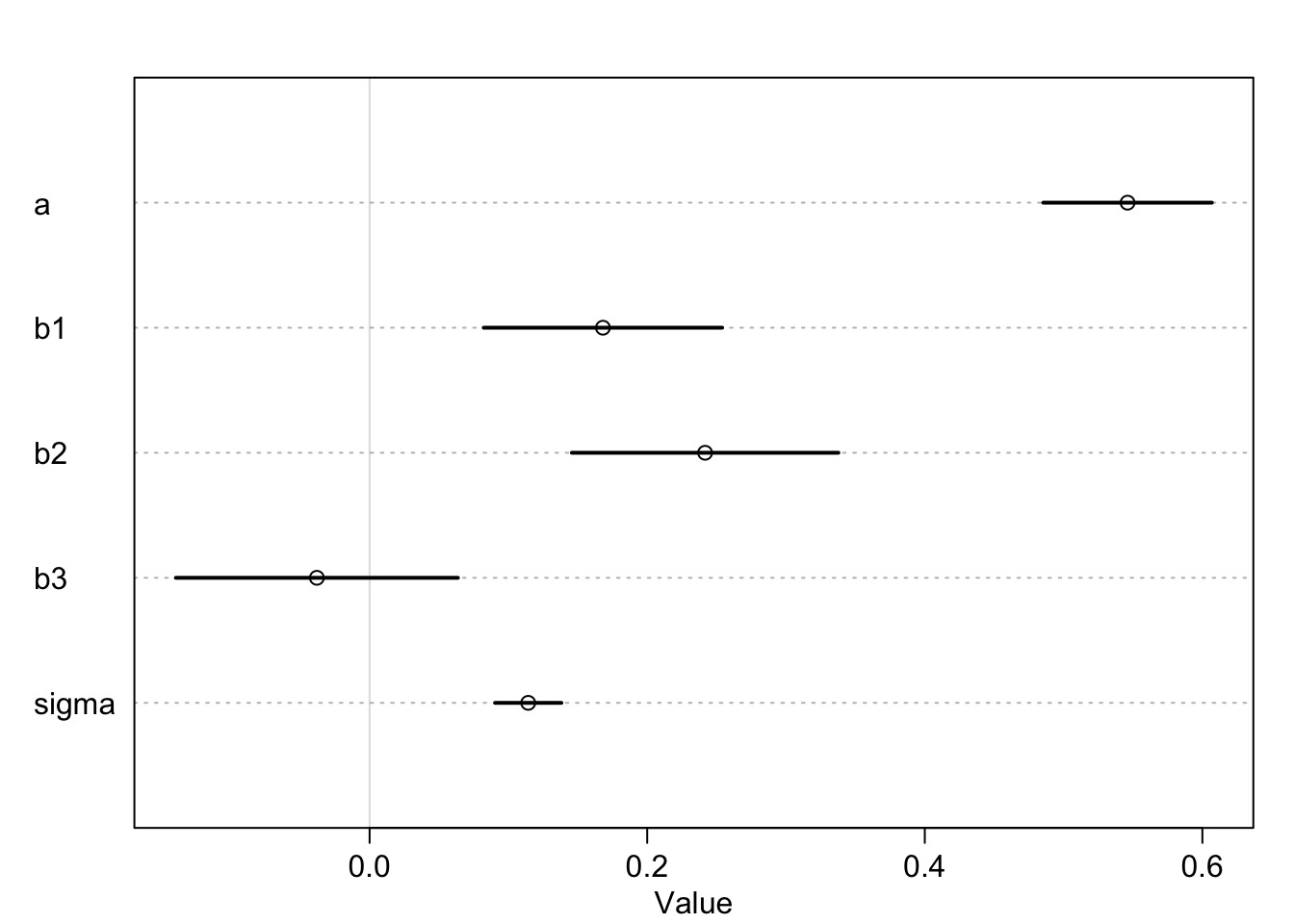
Our Model

mod_med <- alist(
  ## A -> D <- M
  #likelihood 
  D ~ dnorm(mu, sigma),
  
  #data generating processes
  mu <- a + bM*M + bA * A,
  
  # Priors
  a ~ dnorm(0, 0.5),
  bM ~ dnorm(0, 0.5),
  bA ~ dnorm(0, 0.5),
  sigma ~ dunif(0,10),
  
  ## A -> M
  #likelihood 
  M ~ dnorm(mu_m, sigma_m),
  
  #data generating processes
  mu_m <- a_m + bMA*A,
  
  # Priors
  a_m ~ dnorm(0, 0.5),
  bMA ~ dnorm(0, 0.5),
  sigma_m ~ dunif(0,10)

)

fit_med <- quap(mod_med, data=WaffleDivorce)

Calculating Direct and Indirect Effects

Direct: bA
Indirect: bMA x bM
Total = bA + bMA x bM

Calculate and Visualize

We can draw coefficients and calculate using our DAG

coef_med <- tidy_draws(fit_med) |>
  mutate(direct = bA,
         indirect = bMA * bM,
         total = direct + indirect) |>
  select(.draw, total, direct, indirect)

Is there Mediation here?

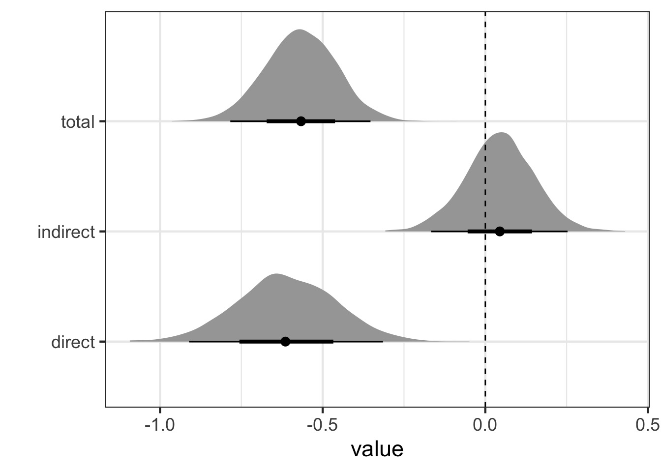
Code

ggplot(coef_med |> pivot_longer(-.draw),
       aes(x = value, y = name)) +
  stat_halfeye() +
  geom_vline(xintercept = 0, lty = 2) +
  labs(y="")

Today’s Outline

Multiple Predictors in a Bayesian Framework
Evaluating a Model with Multiple Predictors
Testing Mediation
Categorical Variables

Categorical Variables

Lots of ways to write models with categorical variables
We all hate R’s treatment contrasts
Two main ways to write a model

Categorical Model Construction

Code each level as 1 or 0 if present/absent
- Need to have one baseline level
- Treatment contrasts!
- Y <- a + b * x_is_level
Index your categories
- Need to convert factors to levels with as.numeric()
- y <- a[level]

Monkies and Milk

Monkies and Milk Production

data(milk)
head(milk)

             clade            species kcal.per.g perc.fat perc.protein
1    Strepsirrhine     Eulemur fulvus       0.49    16.60        15.42
2    Strepsirrhine           E macaco       0.51    19.27        16.91
3    Strepsirrhine           E mongoz       0.46    14.11        16.85
4    Strepsirrhine      E rubriventer       0.48    14.91        13.18
5    Strepsirrhine        Lemur catta       0.60    27.28        19.50
6 New World Monkey Alouatta seniculus       0.47    21.22        23.58
  perc.lactose mass neocortex.perc
1        67.98 1.95          55.16
2        63.82 2.09             NA
3        69.04 2.51             NA
4        71.91 1.62             NA
5        53.22 2.19             NA
6        55.20 5.25          64.54

To easily make Variables

mmat <- model.matrix.default(mass ~ clade, data=milk)
colnames(mmat) <- c("Ape", "New_World_Monkey", "Old_World_Monkey", "Strepsirrhine")
milk <- cbind(milk, mmat)

head(mmat)

  Ape New_World_Monkey Old_World_Monkey Strepsirrhine
1   1                0                0             1
2   1                0                0             1
3   1                0                0             1
4   1                0                0             1
5   1                0                0             1
6   1                1                0             0

Original Milk Model

milk_mod_1 <- alist(
  kcal.per.g ~ dnorm(mu, sigma),
  
  mu <- a*Ape + b1*New_World_Monkey +
    b2*Old_World_Monkey + b3*Strepsirrhine,
  
  a ~ dnorm(0.6, 10),
  b1 ~ dnorm(0,1),
  b2 ~ dnorm(0,1),
  b3 ~ dnorm(0,1),
  sigma ~ dexp(1)
)

milk_fit_1 <- quap(milk_mod_1, data=milk)

Milk Coefs: What does a and b mean?

To get the New World mean…

samp_milk <- extract.samples(milk_fit_1)

new_world <- samp_milk$a + samp_milk$b1

#Deviation from Ape
HPDI(samp_milk$b1)

     |0.89      0.89| 
0.08156998 0.24964529

#New World Monkies
HPDI(new_world)

   |0.89    0.89| 
0.654140 0.773588

A Better Way

milk$clade_idx <- as.numeric(milk$clade)

#A new model
milk_mod_2 <- alist(
  kcal.per.g ~ dnorm(mu, sigma),
  
  #note the indexing!
  mu <- a[clade_idx],
  
  #four priors with one line!
  a[clade_idx] ~ dnorm(0.6, 10),
  sigma ~ dexp(1)
  
)

milk_fit_2 <- quap(milk_mod_2, data=milk)

Compare Results

#New World Monkies
#From Mod1
HPDI(new_world)

   |0.89    0.89| 
0.654140 0.773588

#From Mod2 - note indexing
samp_fit2 <- extract.samples(milk_fit_2)
HPDI(samp_fit2$a[,2])

    |0.89     0.89| 
0.6539256 0.7753170

Exercise

Build a model explaing the kcal.per.g of milk
First try 2 continuous predictors
Add clade
Bonus: Can you make an interaction (try this last)