Information Theory and a Multimodel World

How complex a model do you need to be useful?
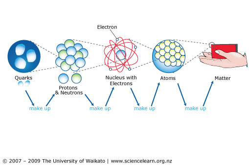
Some models are simple but good enough

More Complex Models are Not Always Better or Right

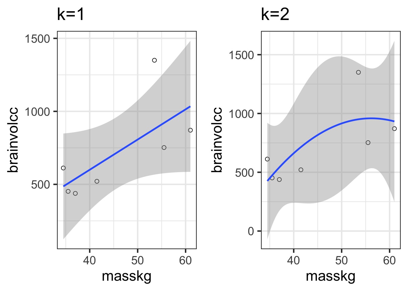
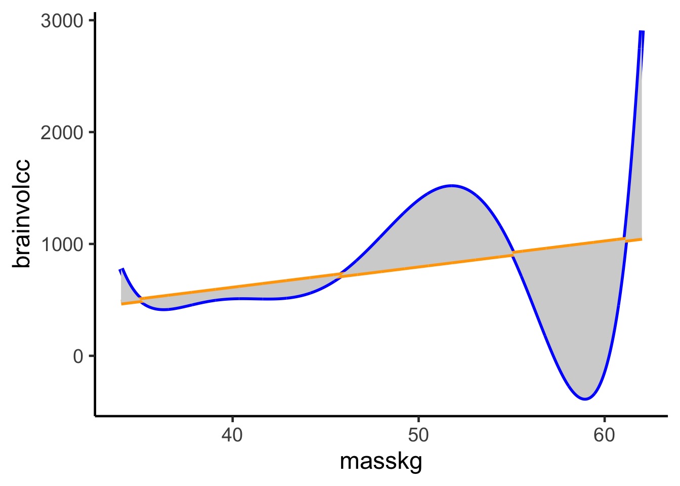
Underfitting

We have explained nothing!
Overfitting
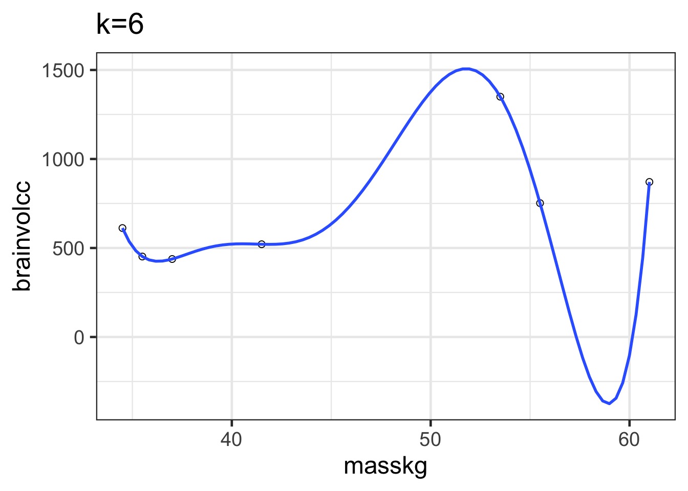
We have perfectly explained this sample
What is the right fit? How do weGet there?
Information Theory and Entropy
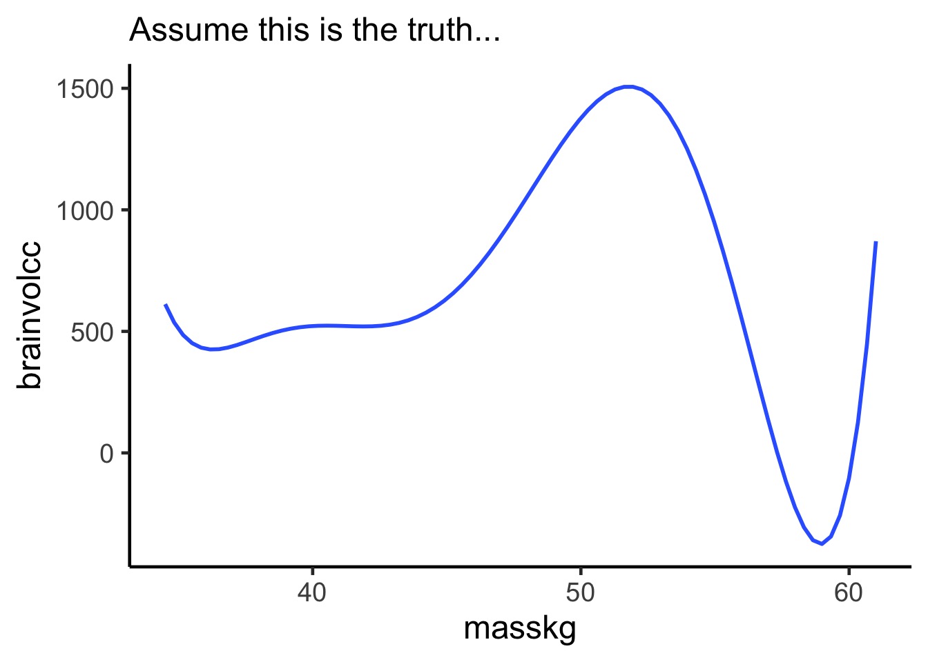
Difference between the truth and a model
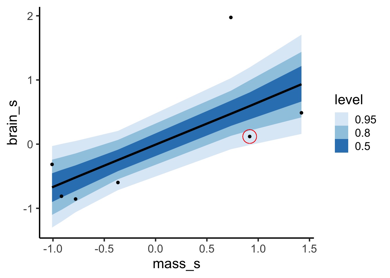
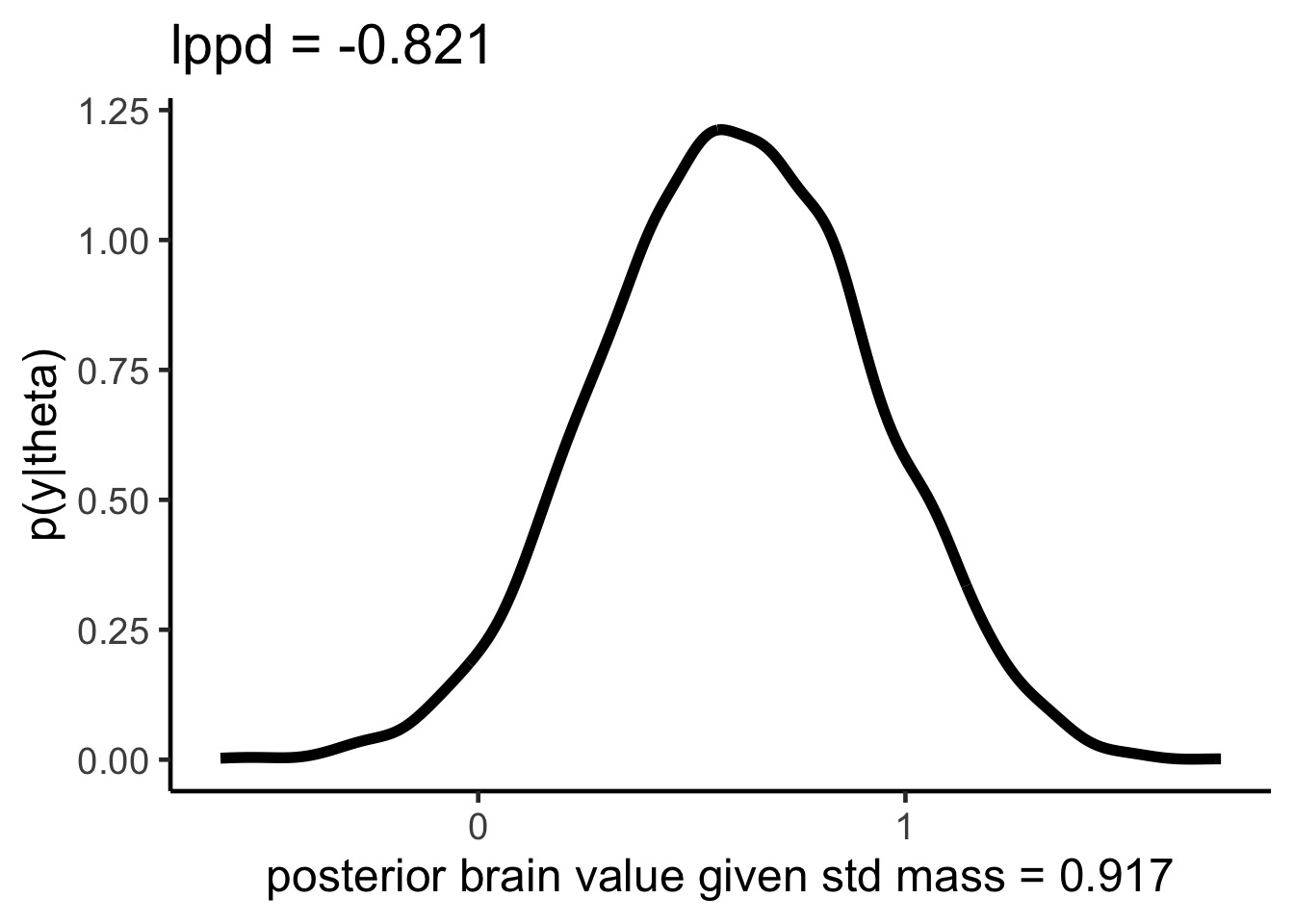
lppd for one point, visually
In and Out of Sample Deviance
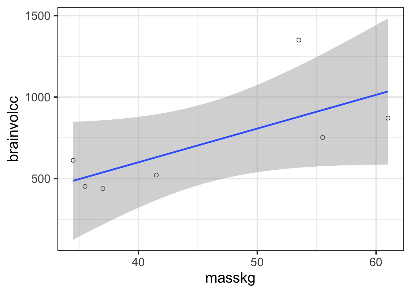
Deviance = -2 * log(dnorm(\(y_i | \mu_i\)))
The deviance of this linear regression is 3.1766285^{5}
In and Out of Sample Deviance
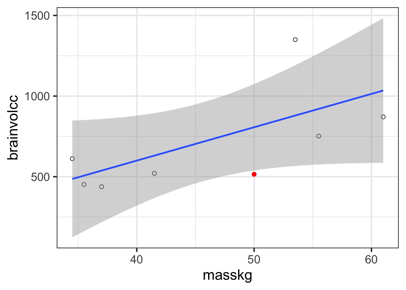
Prediction: 806.8141456, Observe: 515
Deviance: 8.5265838^{4}
In and Out of Sample Deviance
Regularlization
List of 97
$ line :List of 6
..$ colour : chr "black"
..$ linewidth : num 0.773
..$ linetype : num 1
..$ lineend : chr "butt"
..$ arrow : logi FALSE
..$ inherit.blank: logi TRUE
..- attr(*, "class")= chr [1:2] "element_line" "element"
$ rect :List of 5
..$ fill : chr "white"
..$ colour : chr "black"
..$ linewidth : num 0.773
..$ linetype : num 1
..$ inherit.blank: logi TRUE
..- attr(*, "class")= chr [1:2] "element_rect" "element"
$ text :List of 11
..$ family : chr ""
..$ face : chr "plain"
..$ colour : chr "black"
..$ size : num 17
..$ hjust : num 0.5
..$ vjust : num 0.5
..$ angle : num 0
..$ lineheight : num 0.9
..$ margin : 'margin' num [1:4] 0points 0points 0points 0points
.. ..- attr(*, "unit")= int 8
..$ debug : logi FALSE
..$ inherit.blank: logi TRUE
..- attr(*, "class")= chr [1:2] "element_text" "element"
$ title : NULL
$ aspect.ratio : NULL
$ axis.title : NULL
$ axis.title.x :List of 11
..$ family : NULL
..$ face : NULL
..$ colour : NULL
..$ size : NULL
..$ hjust : NULL
..$ vjust : num 1
..$ angle : NULL
..$ lineheight : NULL
..$ margin : 'margin' num [1:4] 4.25points 0points 0points 0points
.. ..- attr(*, "unit")= int 8
..$ debug : NULL
..$ inherit.blank: logi TRUE
..- attr(*, "class")= chr [1:2] "element_text" "element"
$ axis.title.x.top :List of 11
..$ family : NULL
..$ face : NULL
..$ colour : NULL
..$ size : NULL
..$ hjust : NULL
..$ vjust : num 0
..$ angle : NULL
..$ lineheight : NULL
..$ margin : 'margin' num [1:4] 0points 0points 4.25points 0points
.. ..- attr(*, "unit")= int 8
..$ debug : NULL
..$ inherit.blank: logi TRUE
..- attr(*, "class")= chr [1:2] "element_text" "element"
$ axis.title.x.bottom : NULL
$ axis.title.y :List of 11
..$ family : NULL
..$ face : NULL
..$ colour : NULL
..$ size : NULL
..$ hjust : NULL
..$ vjust : num 1
..$ angle : num 90
..$ lineheight : NULL
..$ margin : 'margin' num [1:4] 0points 4.25points 0points 0points
.. ..- attr(*, "unit")= int 8
..$ debug : NULL
..$ inherit.blank: logi TRUE
..- attr(*, "class")= chr [1:2] "element_text" "element"
$ axis.title.y.left : NULL
$ axis.title.y.right :List of 11
..$ family : NULL
..$ face : NULL
..$ colour : NULL
..$ size : NULL
..$ hjust : NULL
..$ vjust : num 0
..$ angle : num -90
..$ lineheight : NULL
..$ margin : 'margin' num [1:4] 0points 0points 0points 4.25points
.. ..- attr(*, "unit")= int 8
..$ debug : NULL
..$ inherit.blank: logi TRUE
..- attr(*, "class")= chr [1:2] "element_text" "element"
$ axis.text :List of 11
..$ family : NULL
..$ face : NULL
..$ colour : chr "grey30"
..$ size : 'rel' num 0.8
..$ hjust : NULL
..$ vjust : NULL
..$ angle : NULL
..$ lineheight : NULL
..$ margin : NULL
..$ debug : NULL
..$ inherit.blank: logi TRUE
..- attr(*, "class")= chr [1:2] "element_text" "element"
$ axis.text.x :List of 11
..$ family : NULL
..$ face : NULL
..$ colour : NULL
..$ size : NULL
..$ hjust : NULL
..$ vjust : num 1
..$ angle : NULL
..$ lineheight : NULL
..$ margin : 'margin' num [1:4] 3.4points 0points 0points 0points
.. ..- attr(*, "unit")= int 8
..$ debug : NULL
..$ inherit.blank: logi TRUE
..- attr(*, "class")= chr [1:2] "element_text" "element"
$ axis.text.x.top :List of 11
..$ family : NULL
..$ face : NULL
..$ colour : NULL
..$ size : NULL
..$ hjust : NULL
..$ vjust : num 0
..$ angle : NULL
..$ lineheight : NULL
..$ margin : 'margin' num [1:4] 0points 0points 3.4points 0points
.. ..- attr(*, "unit")= int 8
..$ debug : NULL
..$ inherit.blank: logi TRUE
..- attr(*, "class")= chr [1:2] "element_text" "element"
$ axis.text.x.bottom : NULL
$ axis.text.y :List of 11
..$ family : NULL
..$ face : NULL
..$ colour : NULL
..$ size : NULL
..$ hjust : num 1
..$ vjust : NULL
..$ angle : NULL
..$ lineheight : NULL
..$ margin : 'margin' num [1:4] 0points 3.4points 0points 0points
.. ..- attr(*, "unit")= int 8
..$ debug : NULL
..$ inherit.blank: logi TRUE
..- attr(*, "class")= chr [1:2] "element_text" "element"
$ axis.text.y.left : NULL
$ axis.text.y.right :List of 11
..$ family : NULL
..$ face : NULL
..$ colour : NULL
..$ size : NULL
..$ hjust : num 0
..$ vjust : NULL
..$ angle : NULL
..$ lineheight : NULL
..$ margin : 'margin' num [1:4] 0points 0points 0points 3.4points
.. ..- attr(*, "unit")= int 8
..$ debug : NULL
..$ inherit.blank: logi TRUE
..- attr(*, "class")= chr [1:2] "element_text" "element"
$ axis.ticks :List of 6
..$ colour : chr "grey20"
..$ linewidth : NULL
..$ linetype : NULL
..$ lineend : NULL
..$ arrow : logi FALSE
..$ inherit.blank: logi TRUE
..- attr(*, "class")= chr [1:2] "element_line" "element"
$ axis.ticks.x : NULL
$ axis.ticks.x.top : NULL
$ axis.ticks.x.bottom : NULL
$ axis.ticks.y : NULL
$ axis.ticks.y.left : NULL
$ axis.ticks.y.right : NULL
$ axis.ticks.length : 'simpleUnit' num 4.25points
..- attr(*, "unit")= int 8
$ axis.ticks.length.x : NULL
$ axis.ticks.length.x.top : NULL
$ axis.ticks.length.x.bottom: NULL
$ axis.ticks.length.y : NULL
$ axis.ticks.length.y.left : NULL
$ axis.ticks.length.y.right : NULL
$ axis.line : list()
..- attr(*, "class")= chr [1:2] "element_blank" "element"
$ axis.line.x : NULL
$ axis.line.x.top : NULL
$ axis.line.x.bottom : NULL
$ axis.line.y : NULL
$ axis.line.y.left : NULL
$ axis.line.y.right : NULL
$ legend.background :List of 5
..$ fill : NULL
..$ colour : logi NA
..$ linewidth : NULL
..$ linetype : NULL
..$ inherit.blank: logi TRUE
..- attr(*, "class")= chr [1:2] "element_rect" "element"
$ legend.margin : 'margin' num [1:4] 8.5points 8.5points 8.5points 8.5points
..- attr(*, "unit")= int 8
$ legend.spacing : 'simpleUnit' num 17points
..- attr(*, "unit")= int 8
$ legend.spacing.x : NULL
$ legend.spacing.y : NULL
$ legend.key :List of 5
..$ fill : chr "white"
..$ colour : logi NA
..$ linewidth : NULL
..$ linetype : NULL
..$ inherit.blank: logi TRUE
..- attr(*, "class")= chr [1:2] "element_rect" "element"
$ legend.key.size : 'simpleUnit' num 1.2lines
..- attr(*, "unit")= int 3
$ legend.key.height : NULL
$ legend.key.width : NULL
$ legend.text :List of 11
..$ family : NULL
..$ face : NULL
..$ colour : NULL
..$ size : 'rel' num 0.8
..$ hjust : NULL
..$ vjust : NULL
..$ angle : NULL
..$ lineheight : NULL
..$ margin : NULL
..$ debug : NULL
..$ inherit.blank: logi TRUE
..- attr(*, "class")= chr [1:2] "element_text" "element"
$ legend.text.align : NULL
$ legend.title :List of 11
..$ family : NULL
..$ face : NULL
..$ colour : NULL
..$ size : NULL
..$ hjust : num 0
..$ vjust : NULL
..$ angle : NULL
..$ lineheight : NULL
..$ margin : NULL
..$ debug : NULL
..$ inherit.blank: logi TRUE
..- attr(*, "class")= chr [1:2] "element_text" "element"
$ legend.title.align : NULL
$ legend.position : chr "right"
$ legend.direction : NULL
$ legend.justification : chr "center"
$ legend.box : NULL
$ legend.box.just : NULL
$ legend.box.margin : 'margin' num [1:4] 0cm 0cm 0cm 0cm
..- attr(*, "unit")= int 1
$ legend.box.background : list()
..- attr(*, "class")= chr [1:2] "element_blank" "element"
$ legend.box.spacing : 'simpleUnit' num 17points
..- attr(*, "unit")= int 8
$ panel.background :List of 5
..$ fill : chr "white"
..$ colour : logi NA
..$ linewidth : NULL
..$ linetype : NULL
..$ inherit.blank: logi TRUE
..- attr(*, "class")= chr [1:2] "element_rect" "element"
$ panel.border :List of 5
..$ fill : logi NA
..$ colour : chr "grey20"
..$ linewidth : NULL
..$ linetype : NULL
..$ inherit.blank: logi TRUE
..- attr(*, "class")= chr [1:2] "element_rect" "element"
$ panel.spacing : 'simpleUnit' num 8.5points
..- attr(*, "unit")= int 8
$ panel.spacing.x : NULL
$ panel.spacing.y : NULL
$ panel.grid :List of 6
..$ colour : chr "grey92"
..$ linewidth : NULL
..$ linetype : NULL
..$ lineend : NULL
..$ arrow : logi FALSE
..$ inherit.blank: logi TRUE
..- attr(*, "class")= chr [1:2] "element_line" "element"
$ panel.grid.major : NULL
$ panel.grid.minor :List of 6
..$ colour : NULL
..$ linewidth : 'rel' num 0.5
..$ linetype : NULL
..$ lineend : NULL
..$ arrow : logi FALSE
..$ inherit.blank: logi TRUE
..- attr(*, "class")= chr [1:2] "element_line" "element"
$ panel.grid.major.x : NULL
$ panel.grid.major.y : NULL
$ panel.grid.minor.x : NULL
$ panel.grid.minor.y : NULL
$ panel.ontop : logi FALSE
$ plot.background :List of 5
..$ fill : NULL
..$ colour : chr "white"
..$ linewidth : NULL
..$ linetype : NULL
..$ inherit.blank: logi TRUE
..- attr(*, "class")= chr [1:2] "element_rect" "element"
$ plot.title :List of 11
..$ family : NULL
..$ face : NULL
..$ colour : NULL
..$ size : 'rel' num 1.2
..$ hjust : num 0
..$ vjust : num 1
..$ angle : NULL
..$ lineheight : NULL
..$ margin : 'margin' num [1:4] 0points 0points 8.5points 0points
.. ..- attr(*, "unit")= int 8
..$ debug : NULL
..$ inherit.blank: logi TRUE
..- attr(*, "class")= chr [1:2] "element_text" "element"
$ plot.title.position : chr "panel"
$ plot.subtitle :List of 11
..$ family : NULL
..$ face : NULL
..$ colour : NULL
..$ size : NULL
..$ hjust : num 0
..$ vjust : num 1
..$ angle : NULL
..$ lineheight : NULL
..$ margin : 'margin' num [1:4] 0points 0points 8.5points 0points
.. ..- attr(*, "unit")= int 8
..$ debug : NULL
..$ inherit.blank: logi TRUE
..- attr(*, "class")= chr [1:2] "element_text" "element"
$ plot.caption :List of 11
..$ family : NULL
..$ face : NULL
..$ colour : NULL
..$ size : 'rel' num 0.8
..$ hjust : num 1
..$ vjust : num 1
..$ angle : NULL
..$ lineheight : NULL
..$ margin : 'margin' num [1:4] 8.5points 0points 0points 0points
.. ..- attr(*, "unit")= int 8
..$ debug : NULL
..$ inherit.blank: logi TRUE
..- attr(*, "class")= chr [1:2] "element_text" "element"
$ plot.caption.position : chr "panel"
$ plot.tag :List of 11
..$ family : NULL
..$ face : NULL
..$ colour : NULL
..$ size : 'rel' num 1.2
..$ hjust : num 0.5
..$ vjust : num 0.5
..$ angle : NULL
..$ lineheight : NULL
..$ margin : NULL
..$ debug : NULL
..$ inherit.blank: logi TRUE
..- attr(*, "class")= chr [1:2] "element_text" "element"
$ plot.tag.position : chr "topleft"
$ plot.margin : 'margin' num [1:4] 8.5points 8.5points 8.5points 8.5points
..- attr(*, "unit")= int 8
$ strip.background :List of 5
..$ fill : chr "grey85"
..$ colour : chr "grey20"
..$ linewidth : NULL
..$ linetype : NULL
..$ inherit.blank: logi TRUE
..- attr(*, "class")= chr [1:2] "element_rect" "element"
$ strip.background.x : NULL
$ strip.background.y : NULL
$ strip.clip : chr "inherit"
$ strip.placement : chr "inside"
$ strip.text :List of 11
..$ family : NULL
..$ face : NULL
..$ colour : chr "grey10"
..$ size : 'rel' num 0.8
..$ hjust : NULL
..$ vjust : NULL
..$ angle : NULL
..$ lineheight : NULL
..$ margin : 'margin' num [1:4] 6.8points 6.8points 6.8points 6.8points
.. ..- attr(*, "unit")= int 8
..$ debug : NULL
..$ inherit.blank: logi TRUE
..- attr(*, "class")= chr [1:2] "element_text" "element"
$ strip.text.x : NULL
$ strip.text.x.bottom : NULL
$ strip.text.x.top : NULL
$ strip.text.y :List of 11
..$ family : NULL
..$ face : NULL
..$ colour : NULL
..$ size : NULL
..$ hjust : NULL
..$ vjust : NULL
..$ angle : num -90
..$ lineheight : NULL
..$ margin : NULL
..$ debug : NULL
..$ inherit.blank: logi TRUE
..- attr(*, "class")= chr [1:2] "element_text" "element"
$ strip.text.y.left :List of 11
..$ family : NULL
..$ face : NULL
..$ colour : NULL
..$ size : NULL
..$ hjust : NULL
..$ vjust : NULL
..$ angle : num 90
..$ lineheight : NULL
..$ margin : NULL
..$ debug : NULL
..$ inherit.blank: logi TRUE
..- attr(*, "class")= chr [1:2] "element_text" "element"
$ strip.text.y.right : NULL
$ strip.switch.pad.grid : 'simpleUnit' num 4.25points
..- attr(*, "unit")= int 8
$ strip.switch.pad.wrap : 'simpleUnit' num 4.25points
..- attr(*, "unit")= int 8
- attr(*, "class")= chr [1:2] "theme" "gg"
- attr(*, "complete")= logi TRUE
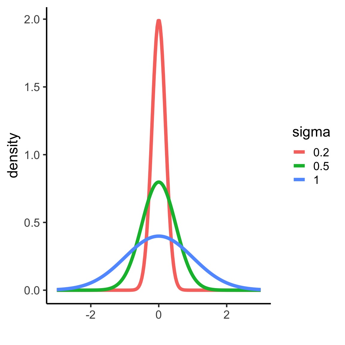
- attr(*, "validate")= logi TRUERegularization means shrinking the prior towards 0
Means data has to work harder to overcome prior
Good way to shrink weak effects with little data, which are often spurious
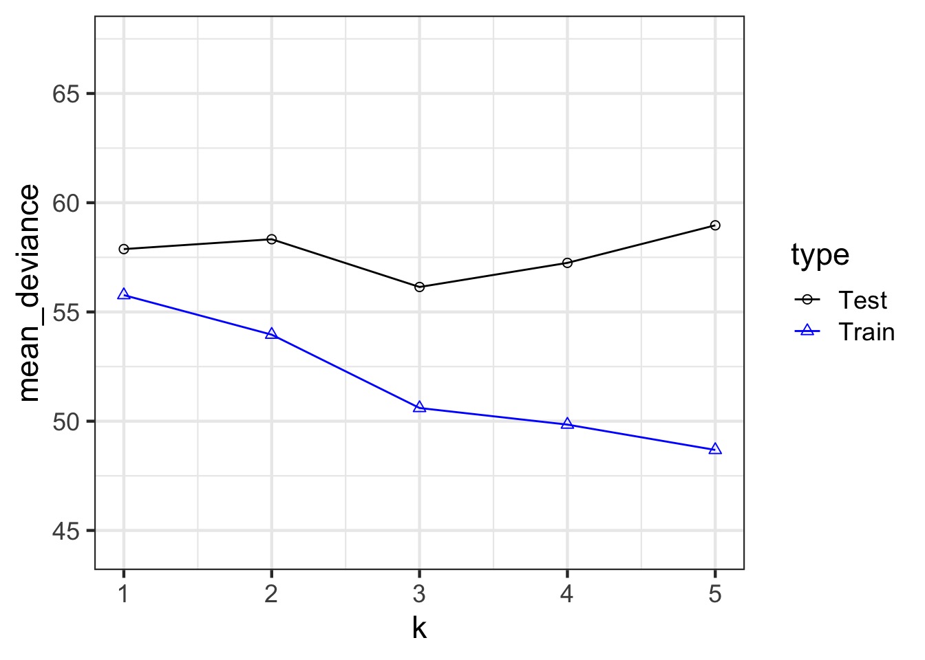
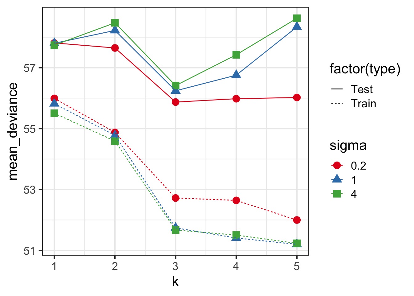
Regularization and Train-Test Deviance
A Criteria Estimating Test Sample Deviance
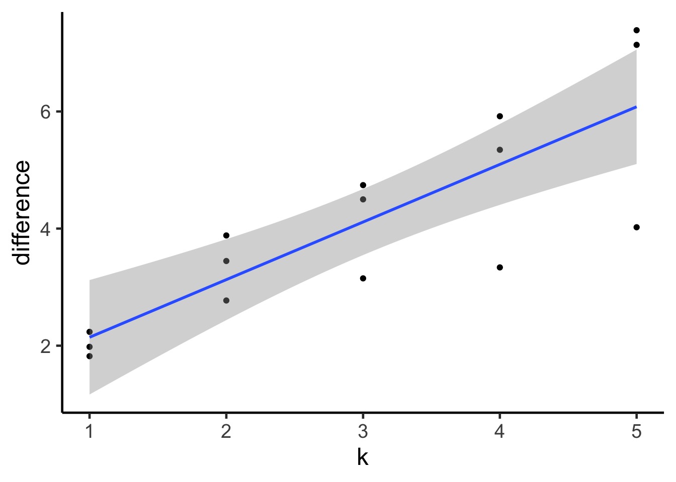
Slope here of 0.98
AIC

So, \(E[D_{test}] = D_{train} + 2K\)
This is Akaike’s Information Criteria (AIC)
\[AIC = Deviance + 2K\]
DIC

\[DIC = 2 \bar{D} - 2 p_D\]
Introducing, the Pareto Distribution
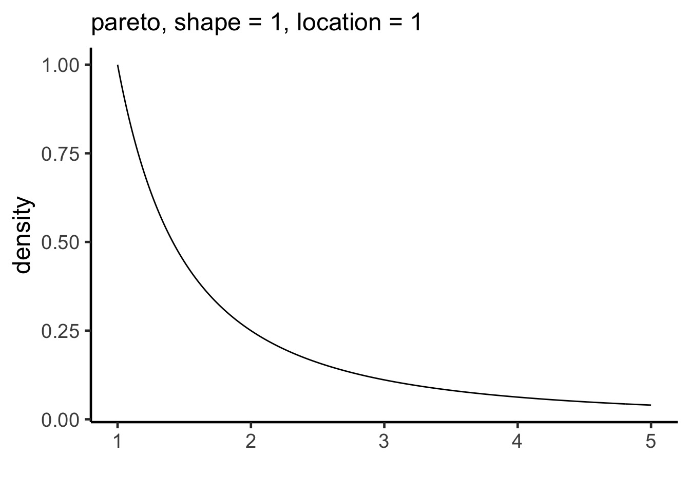
Distribution of importances - 80:20 rule
For each observation, we can use the largest importance value, and calculate a smoothed Pareto curve of weights
PSIS: Pareto Smoothed Importance Sampling
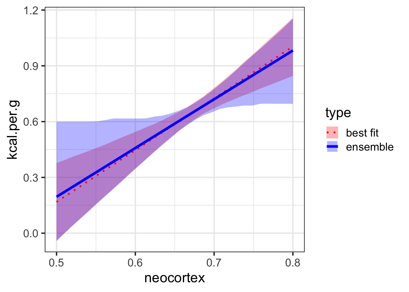
Monkies and Milk

Comparing Models
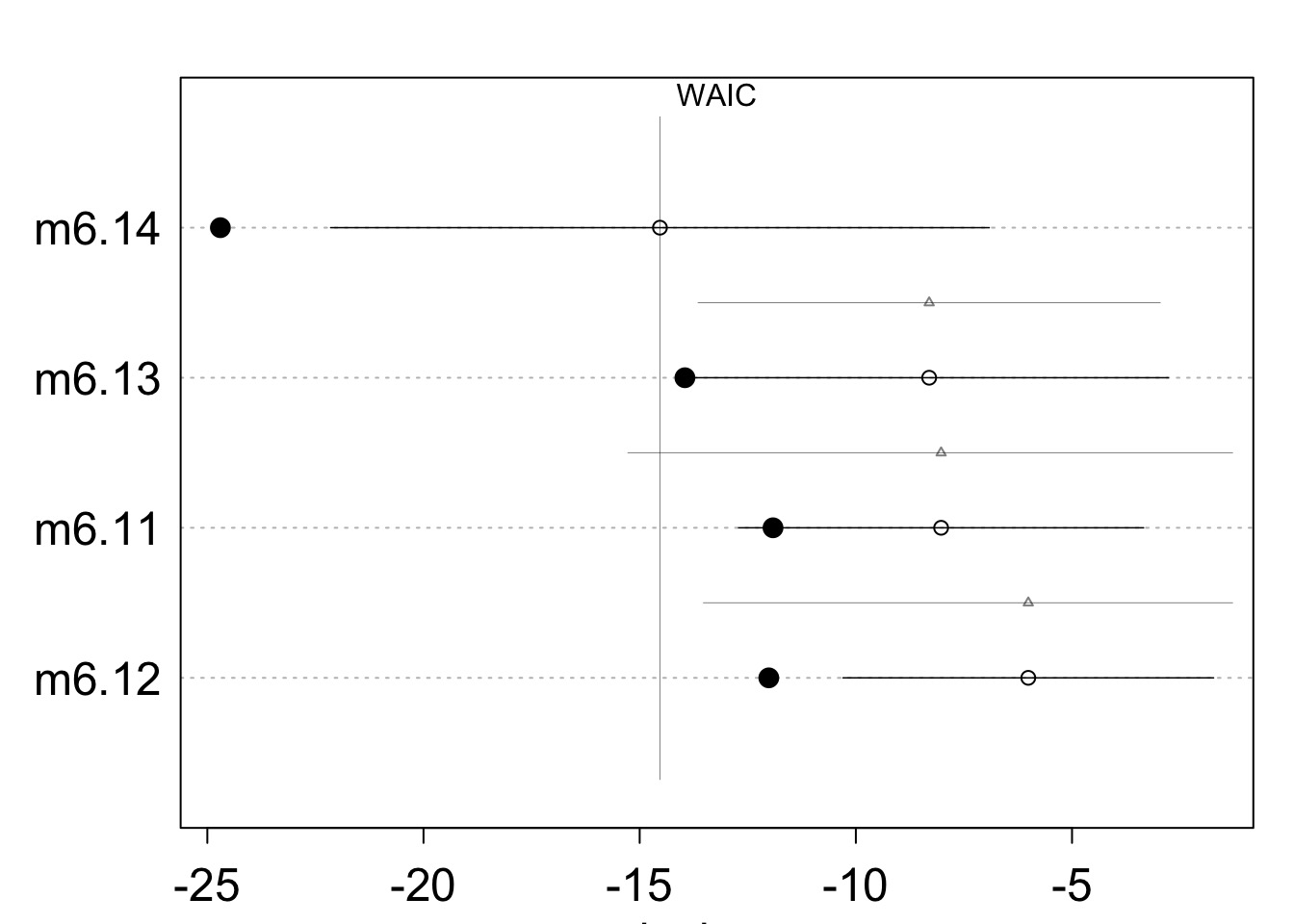
Comparing Models with PSIS

Using WAIC and PSIS to Determine Problem Points
[1] "M mulatta"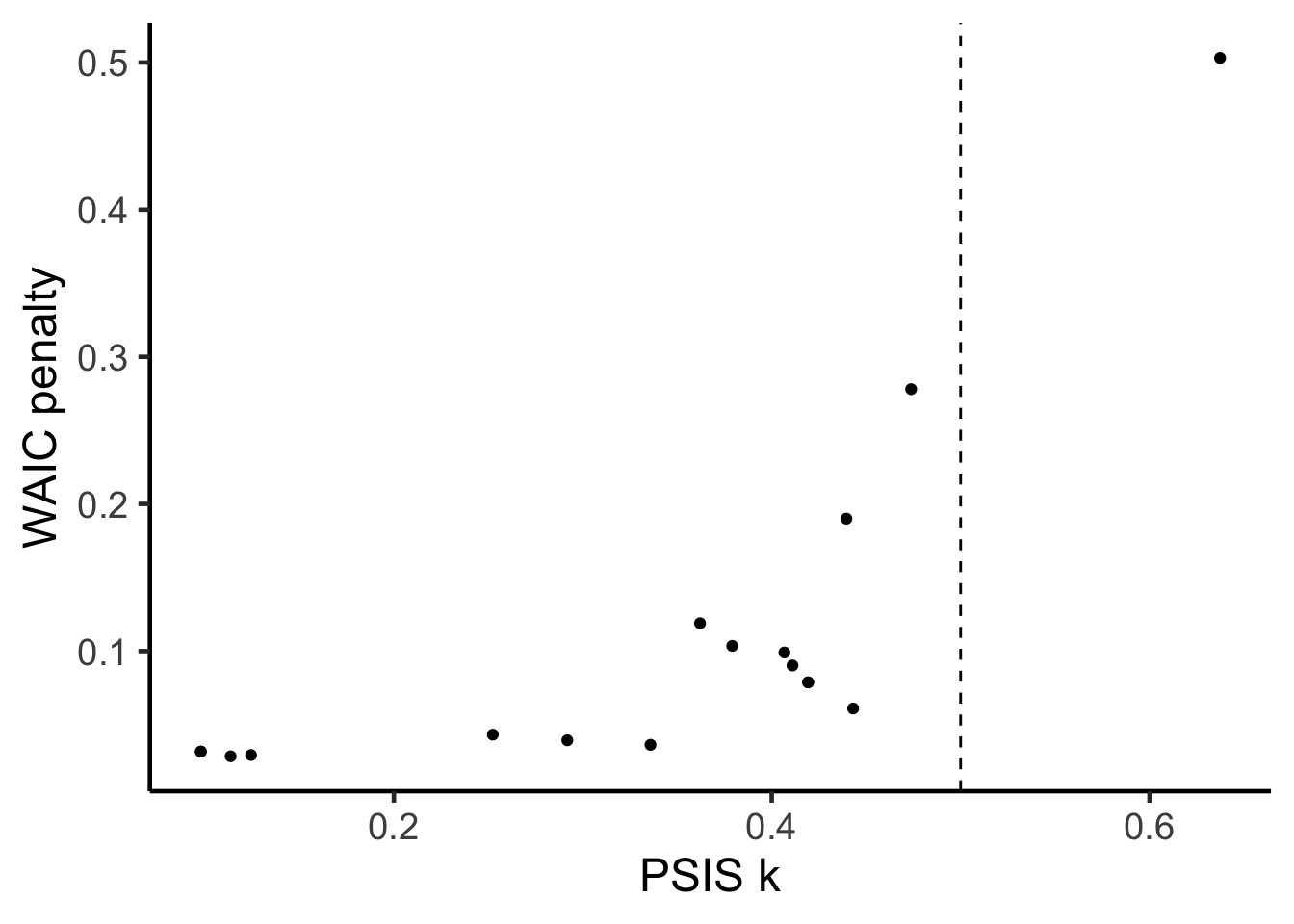


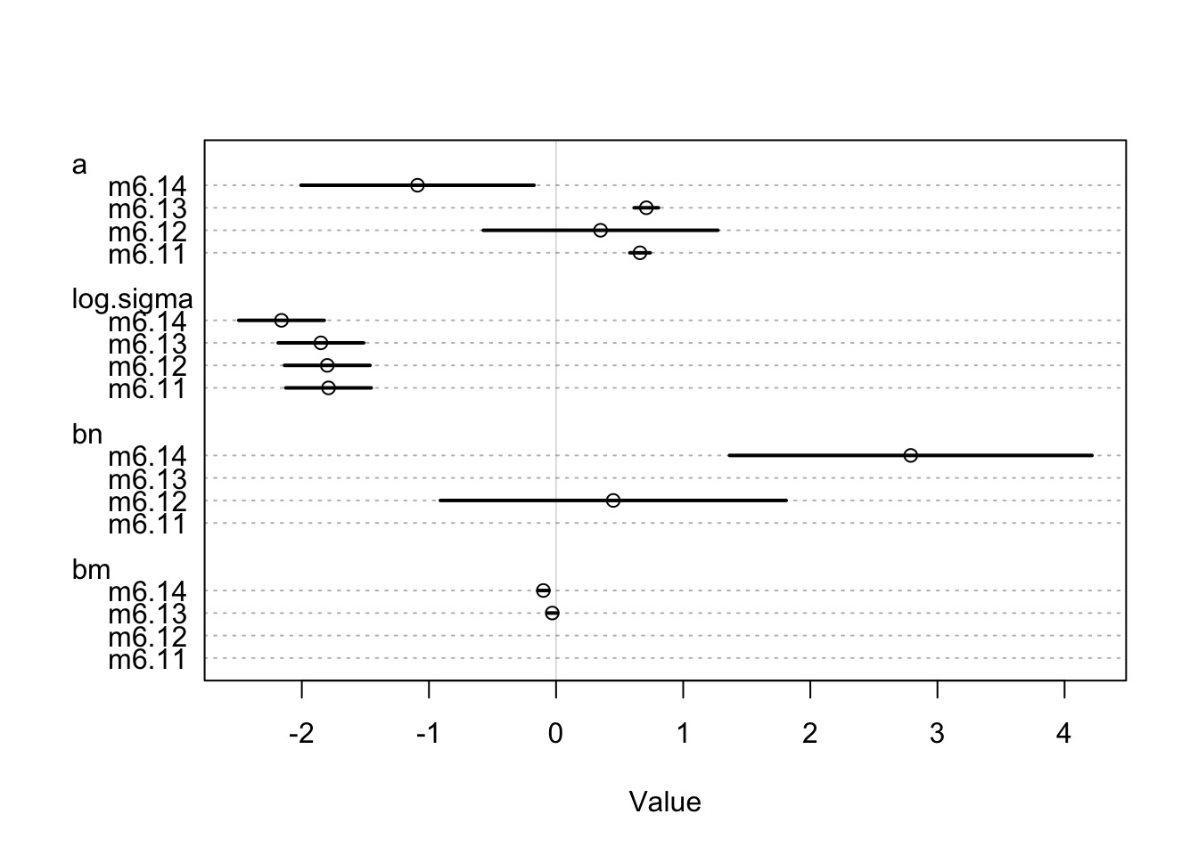
Coefficients
Remember, m6.14 has a 97% WAIC model weight
Making an Ensemble