Missing Data

Three Major Missing Data Problems

1. Meta-analysis as a missing data problem

2. Measurement error in X

3. Missing datapoints

What is Meta-Analysis

• Let’s say you want to summarize results across many studies.
  • Hey, that’s very Bayesian - what is the full posterior?!
• BUT, all you have is means and standard deviations of results.
  • Folk often won’t share raw data.
    
  • Or it’s old! No longer exists!
• Fundamentally, the data is missing.
  - BUT, we have information about it to calculate an effect size

Effect Sizes

• For Group A, you know a mean and SD

• For Group B, you know a mean and SD

• You can then calculate an effect size

  • eg, log ratio = ln(A) - ln(B)
  • Hedge’s G = (A-B)/pooled SD
  • etc…

Can you Survive Extinction?

Does Broad v. Narrow Distribution Size Matter?

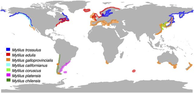
Gaitán-Espitia et al. 2016

Calculating an Effect Size: Log Odds Ratio

• s1 species survive an event in group 1, and e1 go extinct.

• So p1 fraction of species survived an event in group 1 and p2 in group 2

\[lnor = \frac{p1/(1-p1)}{p2/(1-p2)}\]

\[var \: lnor = \sqrt{1/s_1 + 1/e_1 + 1/s_2 + 1/e_2}\]

Summarizing Studies

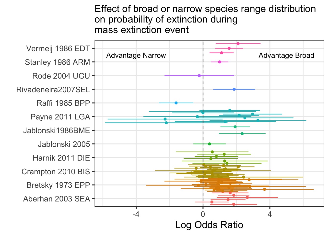
Data from Orzechowski et al. 2015 Global Change Biology

Are these All Just Samples from One Effect Size?

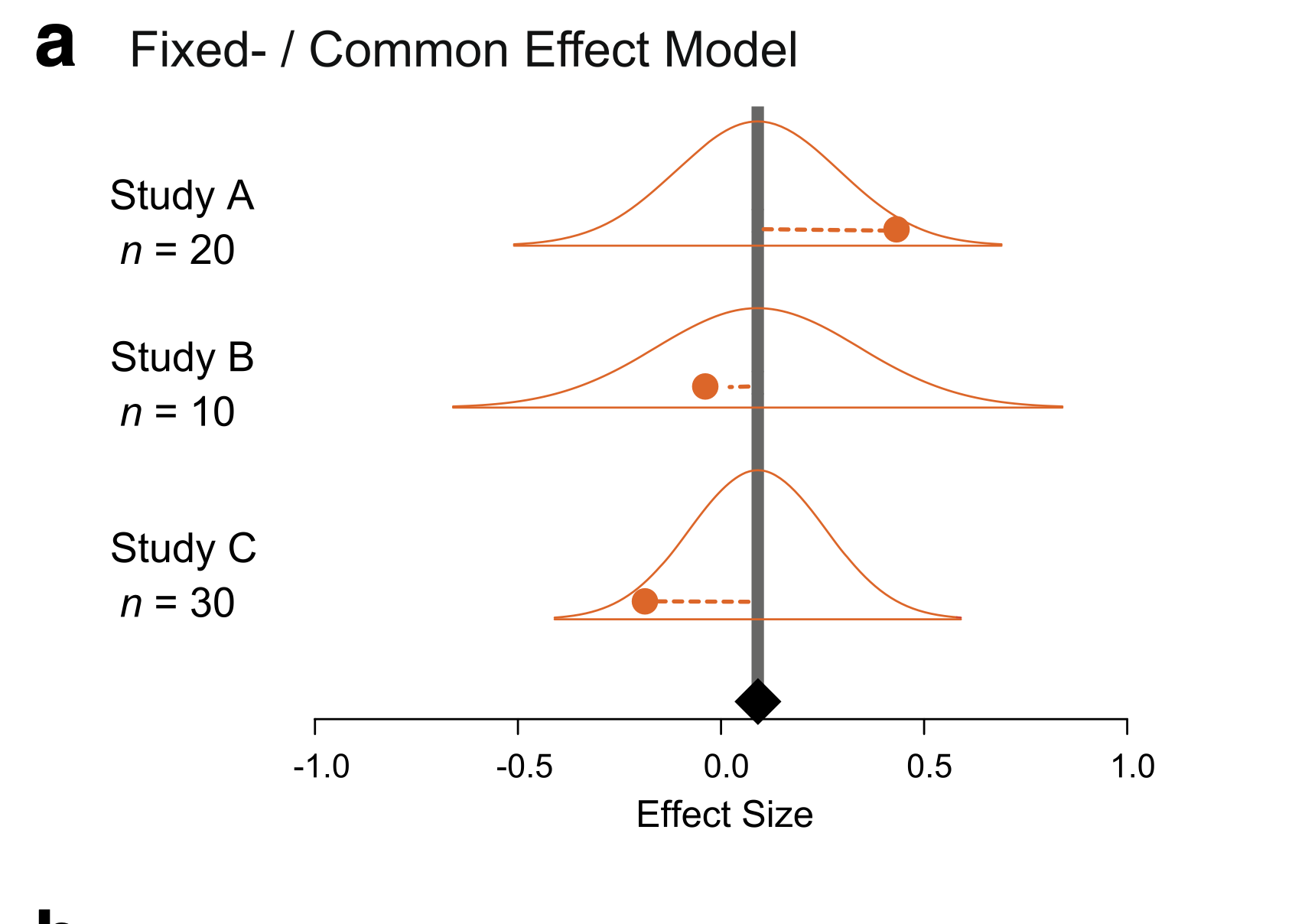Nakagawa et al. 2017

Fixed/Common Effect Meta-Analysis

Likelihood: \[y_i \sim N(\mu, \sigma_i)\]

Prior: \[\mu \sim N(0,1)\]

We have observed \(\sigma_i\).

Bayesian Fit of a FE Meta-Analysis

fe_meta <- quap(
  alist(
    
    # likelihood
    lnorReg ~ dnorm(mu, sd_lnor),
    
    # Prior
    mu ~ dnorm(0, 1)
  ),
  data = ext |>
    select(lnorReg, vlnorReg) |>
    mutate(sd_lnor = sqrt(vlnorReg))
)

What if the Effect Varies from Study to Study?

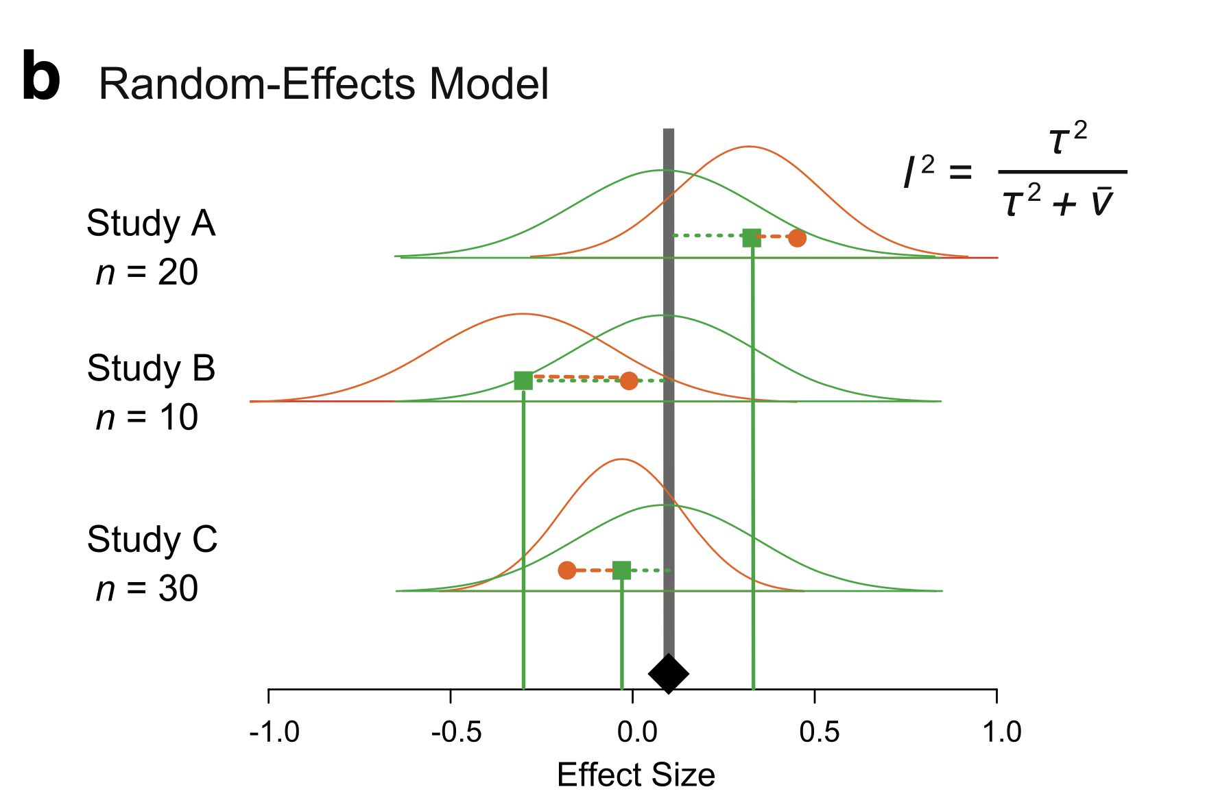
Nakagawa et al. 2017

Random Effects Meta-Analysis

Likelihood: \[y_i \sim N(\theta_i, \sigma_i)\]

Random Effects: \[\theta_i \sim N(\mu, \tau)\]

Prior: \[\mu \sim N(0,1)\] \[\tau \sim halfN(0,2)\]

We have observed \(\sigma_i\) and \(y_i\).

Bayesian Fit of a RE Meta-Analysis

re_meta <- ulam(
  alist(
    
    # likelihood
    lnorReg ~ dnorm(theta[measurement_id], sd_lnor),
    
    # RE
    theta[measurement_id] ~ dnorm(mu, tau),
    
    # Prior
    mu ~ dnorm(0, 1),
    tau ~ dhalfnorm(0,2)
  ),
  data = ext |>
    select(lnorReg, vlnorReg) |>
    mutate(sd_lnor = sqrt(vlnorReg),
           measurement_id = 1:n()),
  chains = 3, log_lik = TRUE
)

Bayesian Fit of a RE Meta-Analysis using NCP

re_meta <- ulam(
  alist(
    
    # likelihood
    lnorReg ~ dnorm(theta, sd_lnor),
    
    # DGP
    theta <- mu + measure_dev[measurement_id],

    # RE
    measure_dev[measurement_id] ~ dnorm(0, tau),
    
    # Prior
    mu ~ dnorm(0, 1),
    tau ~ dhalfnorm(0,2)
  ),
  data = ext |>
    select(lnorReg, vlnorReg) |>
    mutate(sd_lnor = sqrt(vlnorReg),
           measurement_id = 1:n()),
  chains = 3
)

How do BLUPs compare to Means?

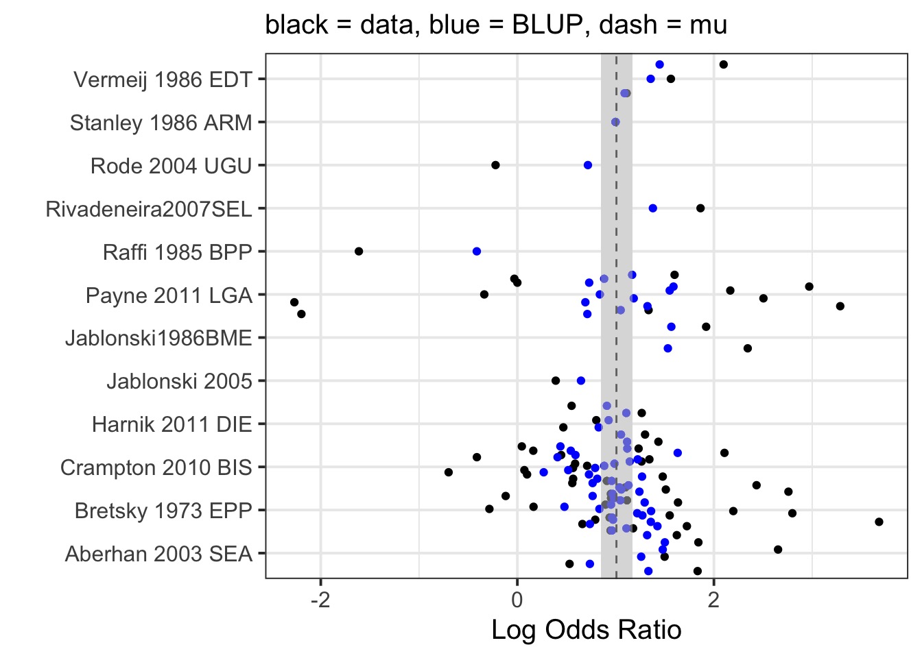
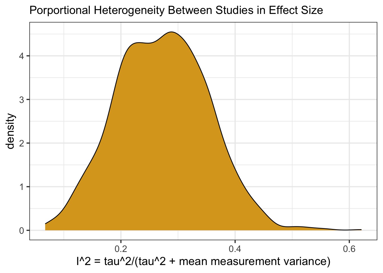
How Much Does and Effect Differ Between Studies?

What If Studies Have Multiple Measurements?

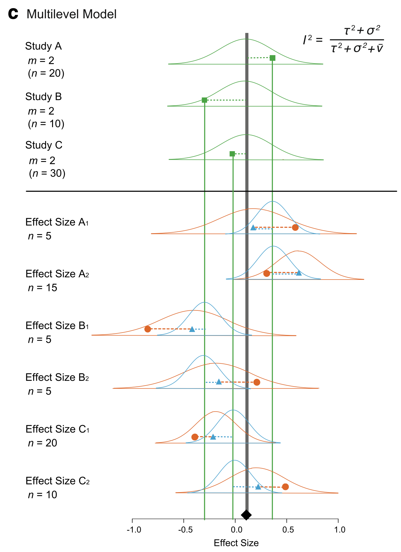
Nakagawa et al. 2017

Multilevel Meta-Analysis

Likelihood: \[y_{ij} \sim N(\theta_{ij}, \sigma_{ij})\]

Random Effects: \[\theta_{ij} \sim N(\psi_i, \omega_{i})\] \[\psi_{i} \sim N(\mu, \tau)\]

Prior: \[\mu \sim N(0,1)\] \[\omega \sim halfN(0,2)\] \[\tau \sim halfN(0,2)\]

We have observed \(\sigma_{ij}\) and \(y_{ij}\).

Bayesian Multilevel Meta-Analysis

multi_meta <- ulam(
  alist(
    
    # likelihood
    lnorReg ~ dnorm(theta[measurement_id], sd_lnor),
    
    # RE
    theta[measurement_id] ~ dnorm(psi[study_id], omega),
    psi[study_id] ~ dnorm(mu, tau),
    
    # Prior
    mu ~ dnorm(0, 1),
    tau ~ dhalfnorm(0,2),
    omega ~ dhalfnorm(0,2)
  ),
  data = ext |>
    select(lnorReg, vlnorReg, study.ID) |>
    mutate(sd_lnor = sqrt(vlnorReg),
           measurement_id = 1:n(),
           study_id = as.numeric(as.factor(study.ID))),
  chains = 4, log_lik = TRUE, iter = 4e3
)

NCP Bayesian Multilevel Meta-Analysis

multi_meta <- ulam(
  alist(
    
    # likelihood
    lnorReg ~ dnorm(theta[measurement_id], sd_lnor),
    
    # DGP
    theta <- mu + measure_dev[measurement_id] + study_dev[study_id],
    
    # RE
    measure_dev[measurement_id] ~ dnorm(0, omega),
    study_dev[study_id] ~ dnorm(0, tau),
    
    # Prior
    mu ~ dnorm(0, 1),
    tau ~ dhalfnorm(0,2),
    omega ~ dhalfnorm(0,2)
  ),
  data = ext |>
    select(lnorReg, vlnorReg, study.ID) |>
    mutate(sd_lnor = sqrt(vlnorReg),
           measurement_id = 1:n(),
           study_id = as.numeric(as.factor(study.ID))),
  chains = 4, log_lik = TRUE, iter = 4e3
)

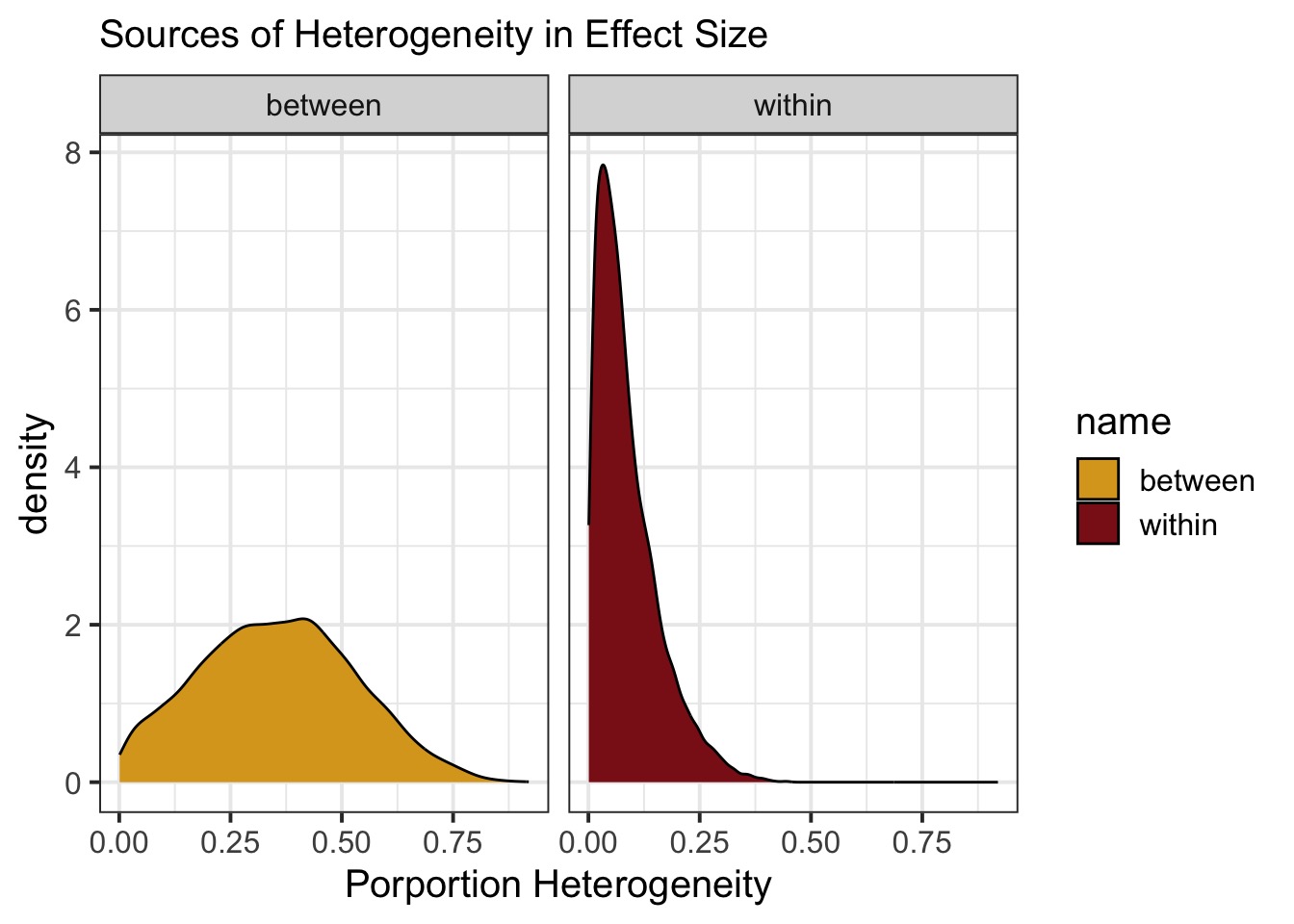
How Much Does and Effect Differ Between Studies?

Bayesian Meta-Analysis

1. When you want to know the state of a field, META-ANALYSIS!

2. We can estimate relationships when we have one more more source of uncertainty in Y.

3. Ask yourself, what are my sources of variation.

   • Meta-regrssion is possible, too!

4. It’s distributions all the way down (NCP can help)!
   

–>

Three Major Missing Data Problems

1. Meta-analysis as a missing data problem

2. Measurement error in X

3. Missing datapoints

Does Measurement Error in Y Bias our Estimates?

Likelihood: \[Y_i \sim N(\hat{Y_i}, \sigma)\]

DGP: \[\hat{Y_i} = \alpha + \beta X_i\]

Oh wait! The measurement error is already there - \(\sigma\) has both process error AND measurement error!

Does Measurement Error in Y Bias our Estimates?

Old School notation: \[Y_i = \alpha + \beta X_i + \epsilon_i + \gamma_i\]

• Error is now decomposed into process error (\(\epsilon_i\)) and measurement error (\(\gamma_i\)).

• Both are normally distributed. Does not affect bias in estimate of \(\beta\)

Does Measurement Error in X Bias our Estimates?

Likelihood: \[Y_i \sim N(\hat{Y_i}, \sigma)\]

DGP in our Model: \[\hat{Y_i} = \alpha + \beta_1 X_i + \beta_1 \nu_i\]

Where, \(\nu_i \sim N(0, \tau)\)

Our estimate of \(\beta_1\) is biased by \(\nu_i\)

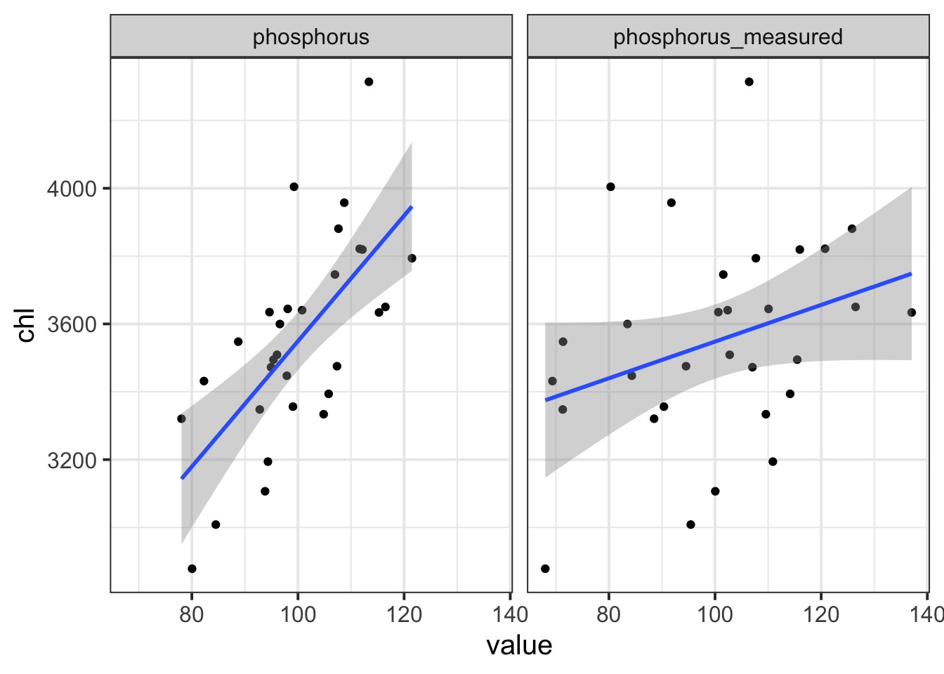
What Does Measurement Error Do

Biggs et al. 2009

Solution

Biggs et al. 2009

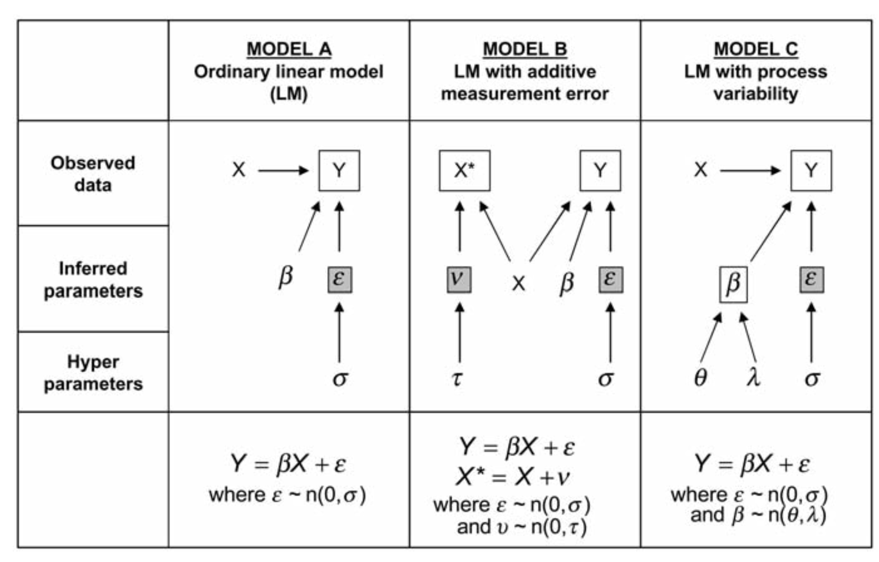
What we Want

Likelihood: \[Y_i \sim N(\hat{Y_i}, \sigma)\]

Measurement Error in X: \[X_i \sim N(\hat{X_i}, \tau)\]

DGP in our Model: \[\hat{Y_i} = \alpha + \beta_1 \hat{X_i}\]

Example: Lakes and Phosphorus Simulation from Biggs et al. 2009

Our Model

Likelihood: \[chl_i \sim N(\hat{chl_i}, \sigma)\]

Measurement Error in X: \[P_i \sim N(\hat{P_i}, \tau)\]

DGP in our Model: \[\hat{chl_i} = \alpha + \beta_1 \hat{P_i}\]

How do we Fit This?

d <- lake_dat |> select(chl, phosphorus_measured) |>
    mutate(chl_s = standardize(chl), 
           phosphorus_measured_s = standardize(phosphorus_measured),
           idx = 1:n())

chl_fit <- ulam(
  alist(
    # likelihood
    chl_s ~ dnorm(chl_hat_s, sigma),
    
    
    # ME
    phosphorus_measured_s ~ dnorm(phosphorus_s[idx], tau),
    phosphorus_s[idx] ~ dnorm( 0, 10 ),
    
    
    # DGP
    chl_hat_s <- a + b*phosphorus_s[idx],
    
    
    # Priors
    a ~ dnorm(0,1),
    b ~ dnorm(0,1),
    sigma ~ dhalfnorm(0,2),
    tau ~ dhalfnorm(0,10)

  ),
  
  data = d,
  
  chains = 3, iter = 6e3)

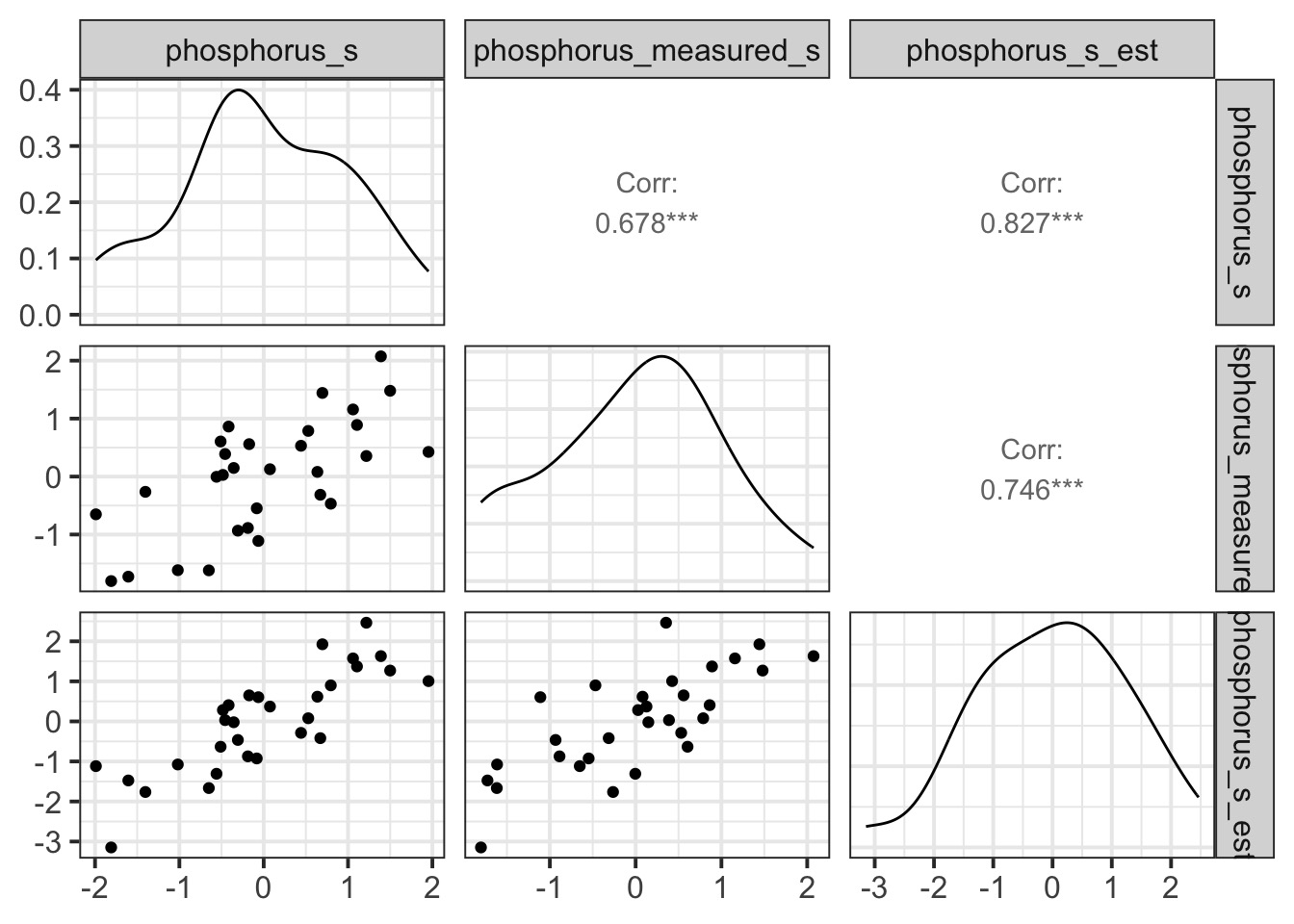
Imputed versus Measured Phosphorus Values

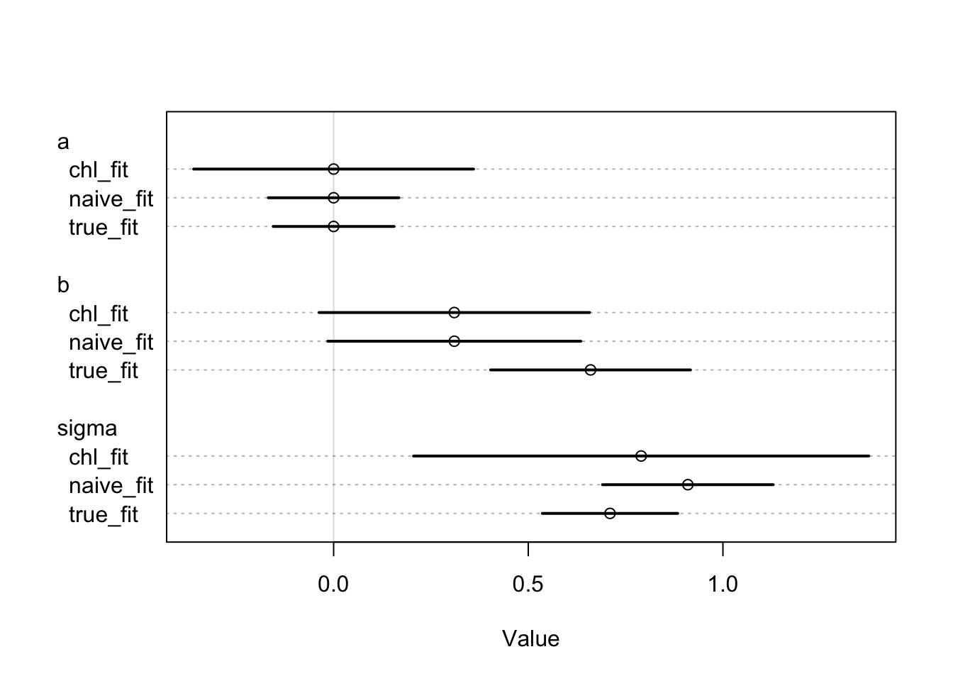
Comparison of Slopes with Versus Without Measurement Error

Going from Standardized to Unstandardized Coefficients

• \[b_{std} = b_{unstd} * sd(x)/sd(y)\]

• \[b_{unstd} = b_{nstd} * sd(y)/sd(x)\]

• \[sd(x_{true}) = sd(x_{with\: error})*\sqrt{1-\tau^2}\]

So on an Unstandardized Scale

          model      mean       sd       5.5%     94.5%
1      True fit 18.182219 3.606099 0.45114870 0.8698756
2    Naieve fit  5.258769 2.822203 0.04396663 0.5739587
3 Corrected Fit       NaN      NaN 0.02855949 0.5823006

Take-Aways

• Measurement error can bias coefficient estimates.
  • This is a HUGE problem
• But, it doesn’t bias fit as much in some cases.
  • More error, potentially more bias, particularly if it is not random.
• What are you seeking to ask? What is important for your project?

Three Major Missing Data Problems

1. Meta-analysis as a missing data problem

2. Measurement error in X

3. Missing datapoints

Previously, We Removed Missing Data from Monkies and Milk

Different Ways for Data to be Missing

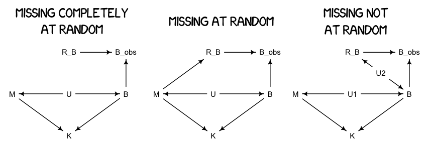
Monkey Prep

data(milk)

d <- milk
d$neocortex.prop <- d$neocortex.perc / 100
d$logmass <- log(d$mass)
dat_list <- list(
    K = standardize( d$kcal.per.g ),
    B = standardize( d$neocortex.prop ),
    M = standardize( d$logmass ) )

A Missing Monkey Model

monkey_mod <- ulam(
    alist(
        # Likelihood
        K ~ dnorm( mu , sigma ),
        
        # DGP
        mu <- a + bB*B + bM*M,
        
        # Missing Data
        B ~ dnorm( nu , sigma_B ),
        
        # Priors
        c(a,nu) ~ dnorm( 0 , 0.5 ),
        c(bB,bM) ~ dnorm( 0, 0.5 ),
        sigma_B ~ dexp( 1 ),
        sigma ~ dexp( 1 )
    ) , data=dat_list , chains=4 , cores=4 )

What were the Values?

                    mean        sd        5.5%      94.5%      rhat  ess_bulk
nu           -0.04714869 0.2049979 -0.37098057  0.2823604 1.0010665 1683.4534
a             0.02805418 0.1626065 -0.22538692  0.2841390 1.0003893 2373.1851
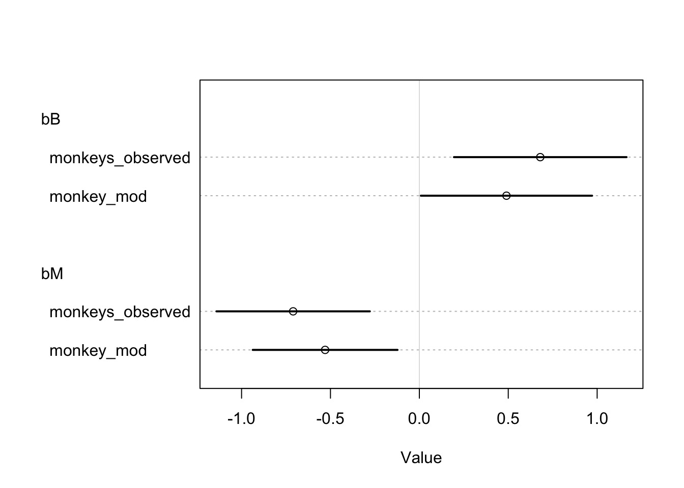
bM           -0.53353005 0.2077682 -0.84813701 -0.1813322 1.0029487 1171.7342
bB            0.49134010 0.2457367  0.07581845  0.8544105 1.0014550  832.7026
sigma_B       1.01533131 0.1754819  0.77362509  1.3229134 1.0004121 1400.3242
sigma         0.84625477 0.1523247  0.63517489  1.1195761 1.0014497 1122.4521
B_impute[1]  -0.57758106 0.8857533 -1.92132945  0.8589375 0.9997388 1772.5683
B_impute[2]  -0.67251768 0.9602740 -2.17094245  0.8504497 1.0006213 2114.2284
B_impute[3]  -0.69251942 0.9334207 -2.13525580  0.8012555 1.0026442 2013.6329
B_impute[4]  -0.26664019 0.8955270 -1.68006795  1.2096898 0.9999199 2595.1109
B_impute[5]   0.46873248 0.9290779 -1.02415665  1.9263149 1.0010083 2607.2185
B_impute[6]  -0.18896418 0.9149612 -1.60841325  1.2467667 1.0014501 2351.7854
B_impute[7]   0.16062658 0.9331044 -1.31401140  1.6316326 1.0014329 2999.6736
B_impute[8]   0.24145252 0.9161032 -1.20155615  1.6830962 1.0018687 2749.1803
B_impute[9]   0.50535876 0.9185386 -0.94126239  1.9197811 1.0010959 2302.9500
B_impute[10] -0.43405382 0.9102278 -1.85549965  1.0841341 1.0040564 2474.1664
B_impute[11] -0.28032590 0.9056276 -1.71838520  1.1071042 0.9995017 2894.9464
B_impute[12]  0.14044318 0.9248727 -1.37572560  1.5707976 1.0025727 2640.2179

Imputing Increases Precision

Missing Data Extravaganza

• We can impute data!

• It’s all just distributions, anyway

• But, be wary of the structure of missingness and how observation error enters the fray