Bayesian Generalized Linear Models

Our Models Until Now

Likelihood:
\(y_i \sim Normal(\mu_i, \sigma)\)

Data Generating Process
\(\mu_i = \alpha + \beta_1 x1_i + \beta_2 x2_i + ...\)

Priors:
\(\alpha \sim Normal(0, 1)\)
\(\beta_j \sim Normal(0, 1)\)
\(\sigma \sim cauchy(0,2)\)

Making the Normal General

Likelihood:
\(y_i \sim Normal(\mu_i, \sigma)\)

Data Generating Process with identity link
f(\(\mu_i) = \alpha + \beta_1 x1_i + \beta_2 x2_i + ...\)

Priors:
…

A Generalized Linear Model

Likelihood:
\(y_i \sim D(\theta_i, ...)\)

Data Generating Process with identity link
f(\(\theta_i) = \alpha + \beta_1 x1_i + \beta_2 x2_i + ...\)

Priors:
…

A Generalized Outline

Why use GLMs? An Intro to Entropy
Logistic Regression
Poisson Regression
Poisson -> Multinomial

What is Maximum Entropy?

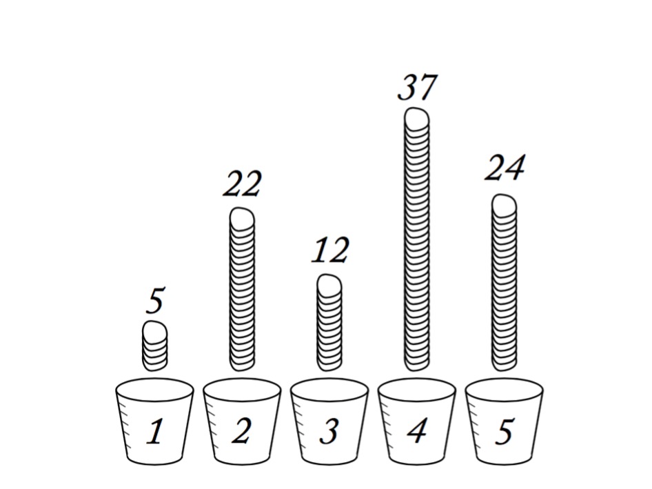
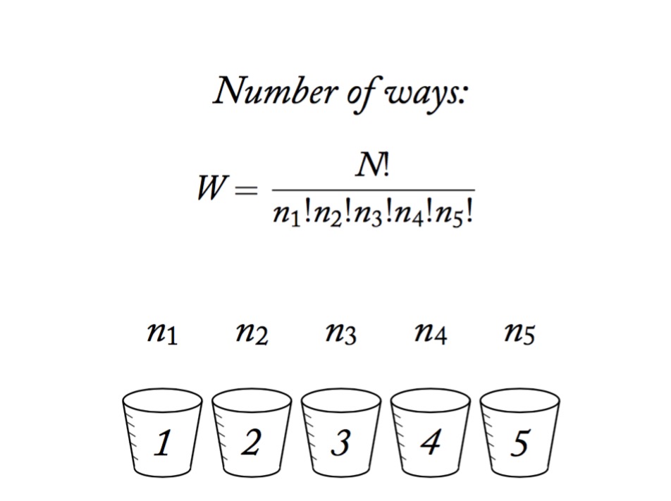
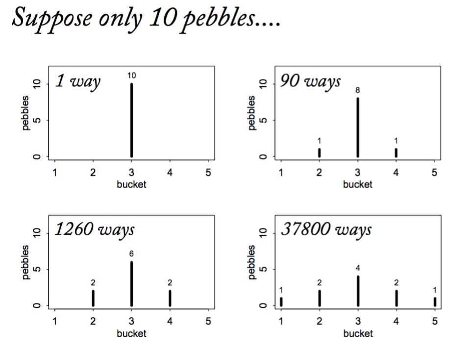
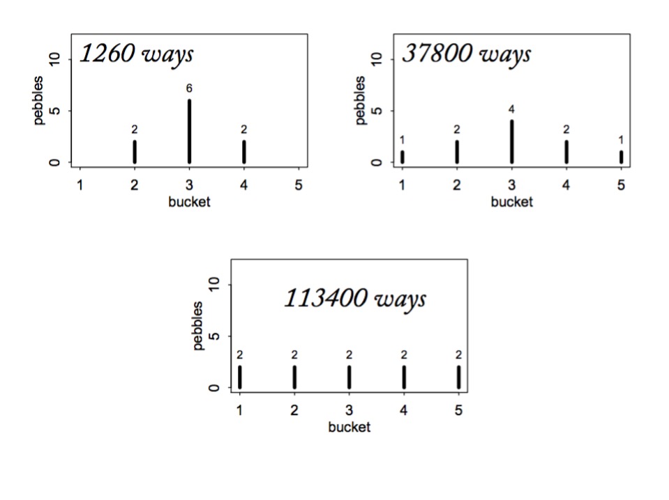
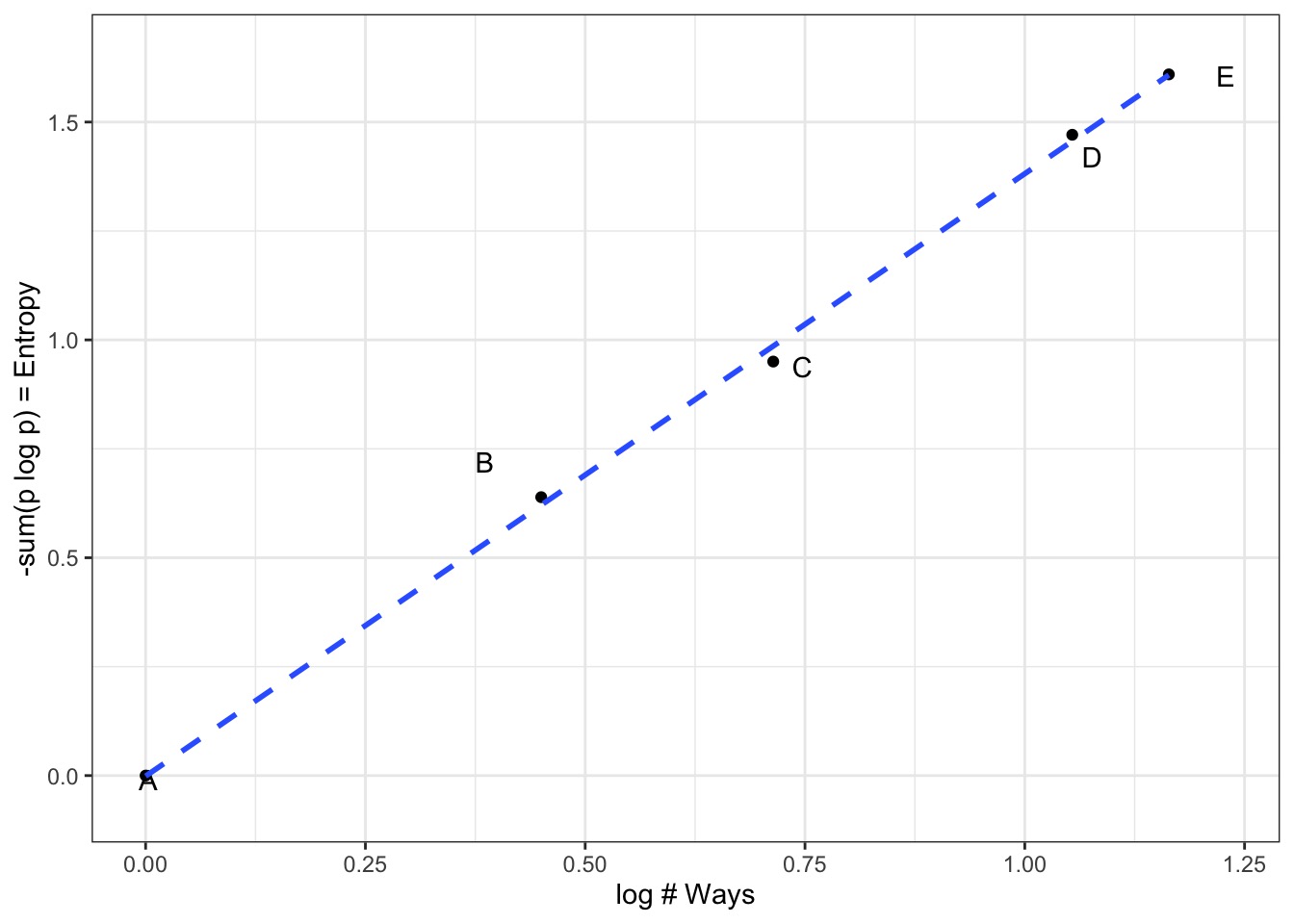
Maximum Entropy Principle

The distribution that can happen the most ways is also the distribution with the biggest information entropy. The distribution with the biggest entropy is the most conservative distribution that obeys its constraints.

-McElreath 2017

Why are we thinking about MaxEnt?

MaxEnt distributions have the widest spread - conservative
Nature tends to favor maximum entropy distributions
- It’s just natural probability
The foundation of Generalized Linear Model Distributions
Leads to useful distributions once we impose constraints

McElreath 2016

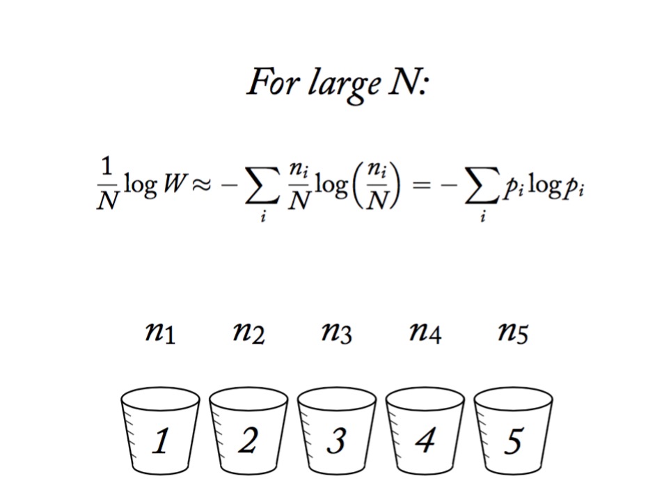
Information Entropy

\[H(p) = - \sum p_i log \, p_i\]

Measure of uncertainty
If more events possible, it increases
Nature finds the distribution with the largest entropy, given constraints of distribution

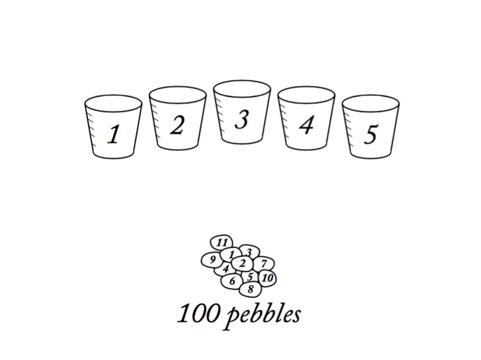
Maximum Entropy and Coin Flips

Let’s say you are flipping a fair (p=0.5) coin twice
What is the maximum entropy distribution of # Heads?
Possible Outcomes: TT, HT, TH, HH
- which leads to 0, 1, 2 heads
Constraint is, with p=0.5, the average outcome is 1 heads

The Binomial Possibilities

TT = p²
HT = p(1-p)
TH = (1-p)p
HH = p²

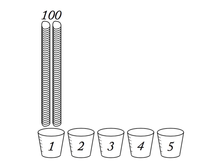
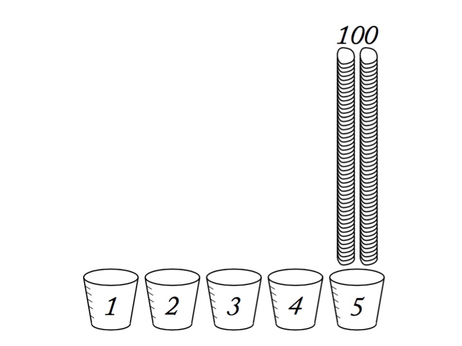
But other distributions are possible

Let’s compare other distributions meeting constraint using Entropy

Remember, we must average 1 Heads, so,
sum(distribution * 0,1,1,2) = 1

\[H = - \sum{p_i log p_i}\]

Distribution	TT, HT, TH, HH	Entropy
Binomial	1/4, 1/4, 1/4, 1/4	1.386
Candiate 1	2/6, 1/6, 1/6, 2/6	1.33
Candiate 2	1/6, 2/6, 2/6, 1/6	1.33
Candiate 3	1/8, 1/2, 1/8, 2/8	1.213

Binomial wins!

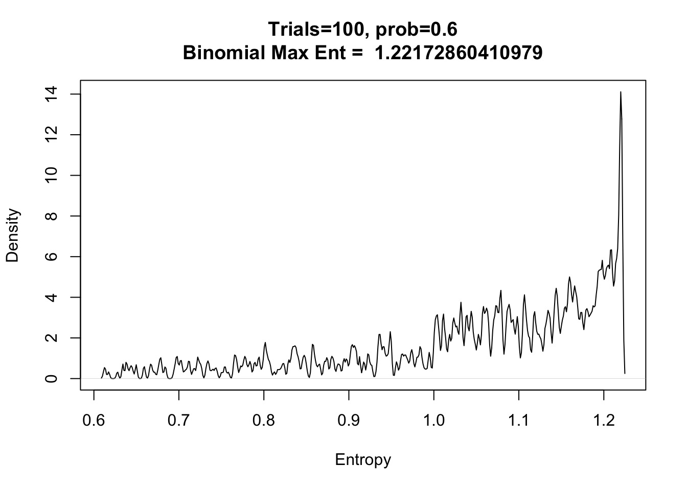
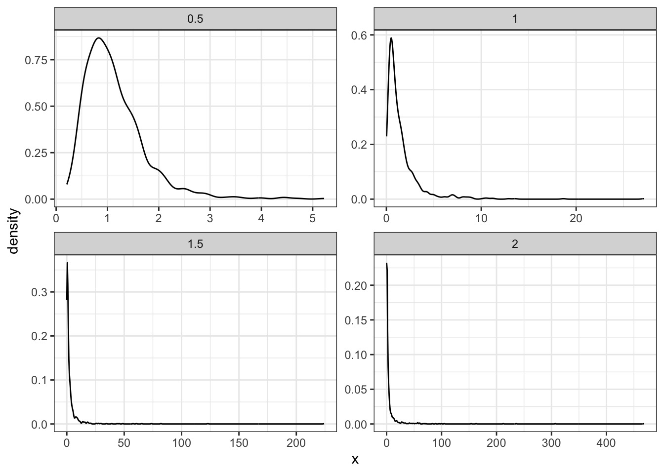
What about other p’s and draws?

Assume 2 draws, p=0.7, make 1000 simulated distributions

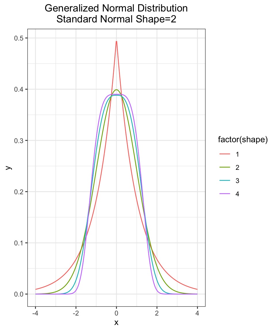
OK, what about the Gaussian?

Constraints: mean, finite variance, unbounded
Lots of possible distributions for normal processes
Flattest distribution given constraints: MaxEnt

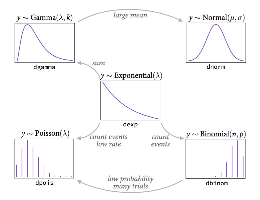
Maximum Entropy Distributions

Constraints	Maxent distribution
Real value in interval	Uniform
Real value, finite variance	Gaussian
Binary events, fixed probability	Binomial
Sum of binomials as n -> inf	Binomial
Non-negative real, has mean	Exponential

How to determine which non-normal distribution is right for you

Use previous table to determine
Bounded values: binomial, beta, Dirchlet
Counts: Poisson, multinomial, geometric
Distances and durations: Exponential, Gamma (survival or event history)
Monsters: Ranks and ordered categories
Mixtures: Beta-binomial, gamma-Poisson, Zero-inflated processes

How Distributions are Coupled

A Generalized Outline

Why use GLMs? An Intro to Entropy
Logistic Regression
Poisson Regression
Poisson -> Multinomial

Our Models Until Now

Likelihood:
\(y_i \sim Normal(\mu_i, \sigma)\)

Data Generating Process
\(\mu_i = \alpha + \beta_1 x1_i + \beta_2 x2_i + ...\)

Priors:
\(\alpha \sim Normal(0, 1)\)
\(\beta_j \sim Normal(0, 1)\)
\(\sigma \sim cauchy(0,2)\)

Binomial Logistic Regression

Likelihood:
\(y_i \sim B(size, p_i)\)

Data Generating Process with identity link
logit(\(p_i) = \alpha + \beta_1 x1_i + \beta_2 x2_i + ...\)

Priors:
…

Why Binomial Logistic Regression

Allows us to predict absolute probability of something occuring
Allows us to determing relative change in risk due to predictors

Why a Logit Link?

McElreath 2016

Meaning of Logit Coefficients

\[logit(p_i) = log \frac{p_i}{1-p_i} = \alpha + \beta x_i\]

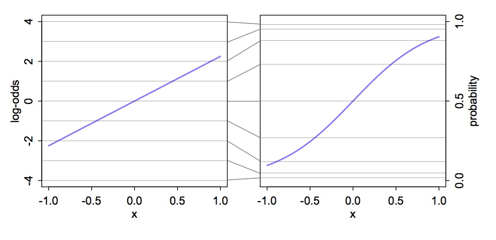
\(\frac{p_i}{1-p_i}\) is odds of something happening
\(\beta\) is change in log odds per one unit change in \(x_i\)
- exp(\(\beta\)) is change in odds
- Change in relative risk
\(p_i\) is absolute probability of something happening
- logistic(\(\alpha + \beta x_i\)) = probability
- To evaluate change in probability, choose two different \(x_i\) values

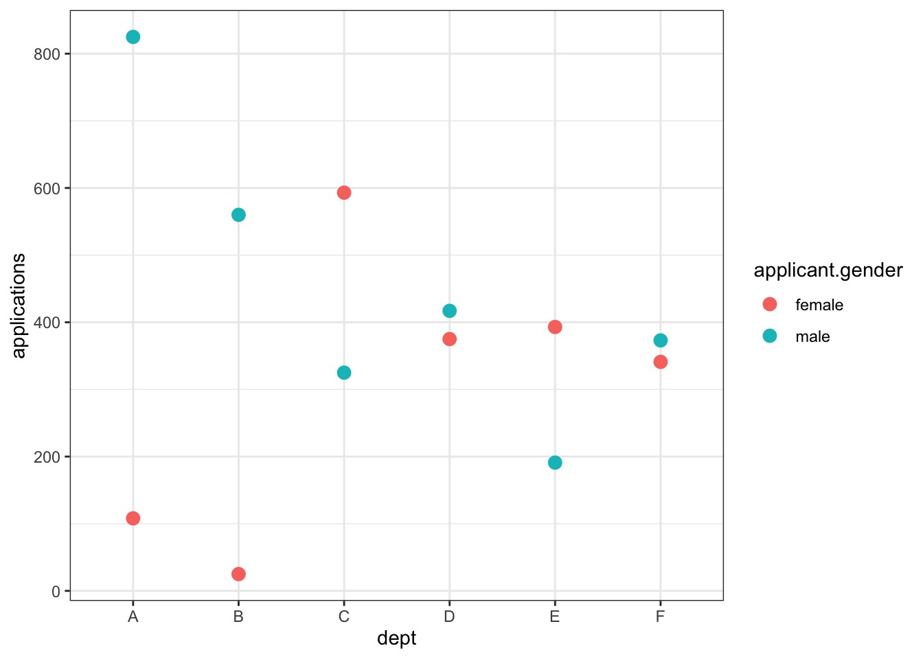
Binomial GLM in Action: Gender Discrimination in Graduate Admissions

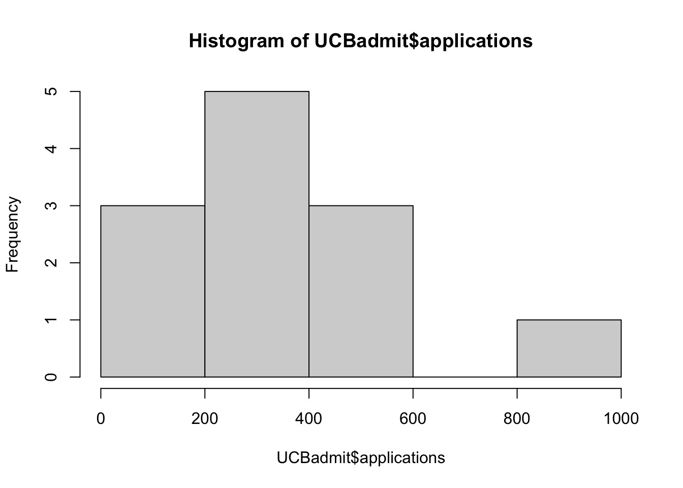
Our data: Berkeley in 1973

data(UCBadmit)
head(UCBadmit)

  dept applicant.gender admit reject applications
1    A             male   512    313          825
2    A           female    89     19          108
3    B             male   353    207          560
4    B           female    17      8           25
5    C             male   120    205          325
6    C           female   202    391          593

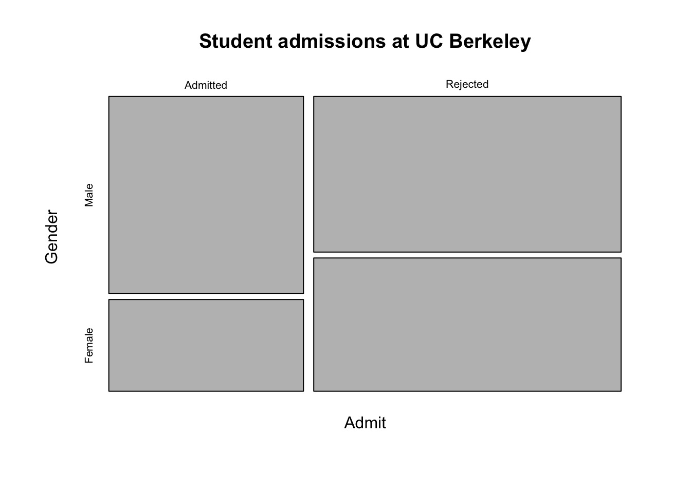
The Gender Gap

          Gender
Admit      Male Female
  Admitted 1198    557
  Rejected 1493   1278

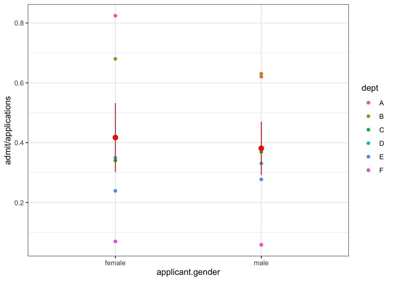
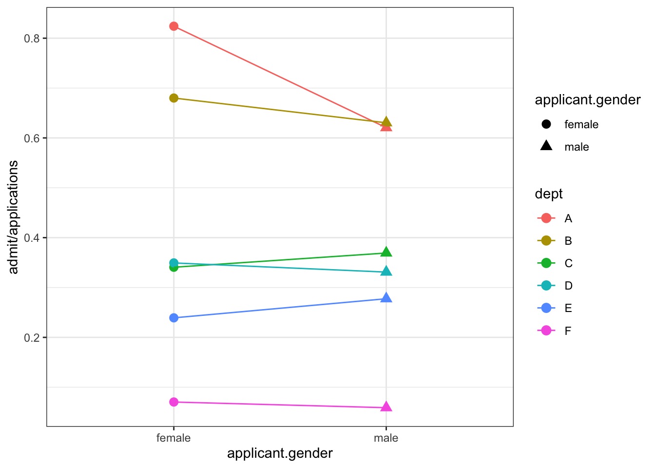
Doesn’t Look like a Gender Gap if we Factor In Department…

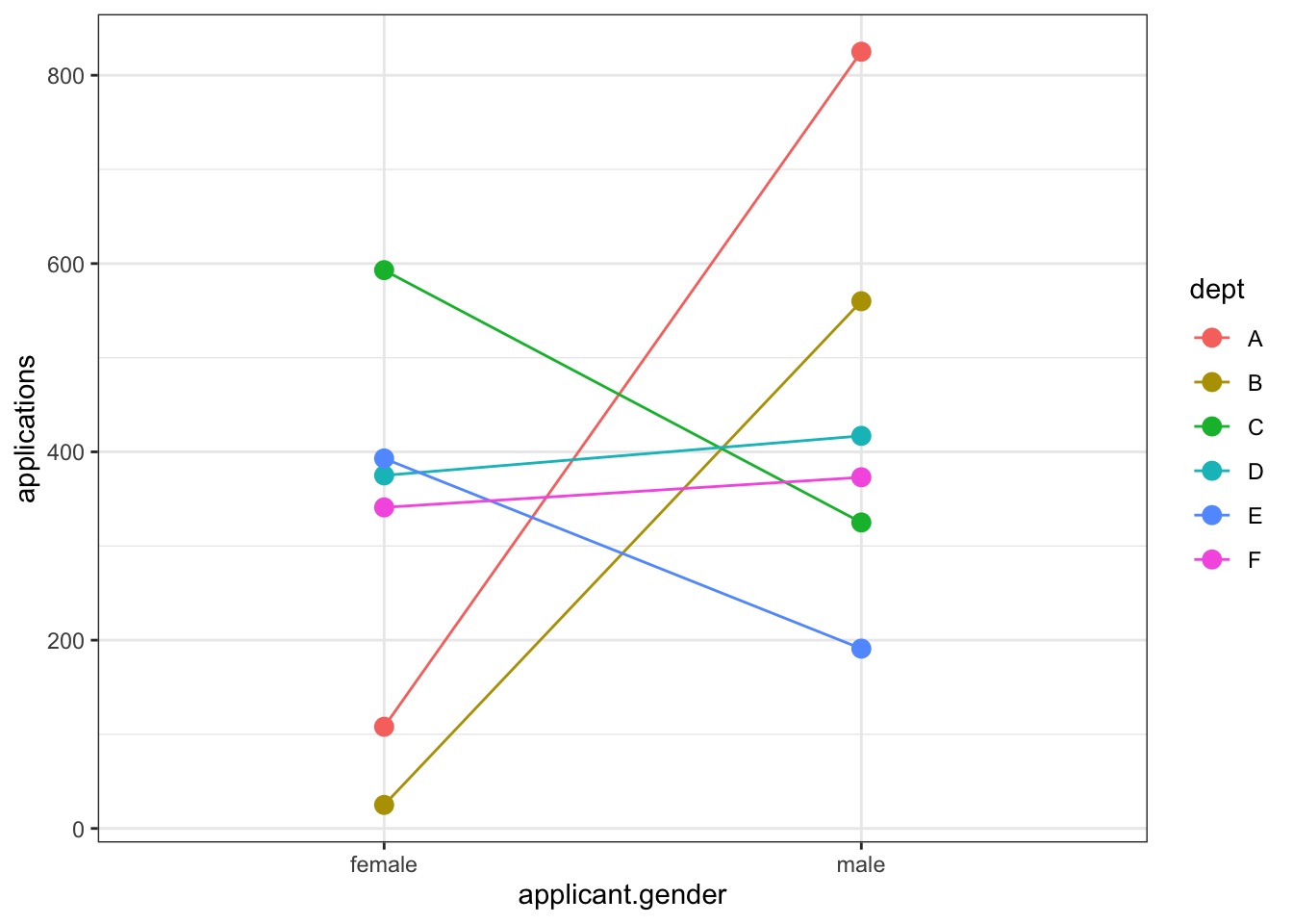
But Gender -> Department Applied To

Porportion Admitted by Department…

What model would you build?

  dept applicant.gender admit reject applications
1    A             male   512    313          825
2    A           female    89     19          108
3    B             male   353    207          560
4    B           female    17      8           25
5    C             male   120    205          325
6    C           female   202    391          593

Mediation Model

Gender influences where you apply to. Department mediates gender to admission relationship.

One Model

#female = 1, male = 2
UCBadmit <-  UCBadmit |>
  mutate(gender = as.numeric(applicant.gender),
         dept_id = as.numeric(dept))

mod_gender <- alist(
  #likelihood
  admit ~ dbinom(applications, p),
  
  #Data generating process
  logit(p) <- a[gender] + delta[dept_id],
  
  #priors
  a[gender] ~ dnorm(0,1),
  delta[dept_id] ~ dnorm(0,1)
)

fit_gender <- quap(mod_gender, UCBadmit)

What do Priors Imply in a GLMS?

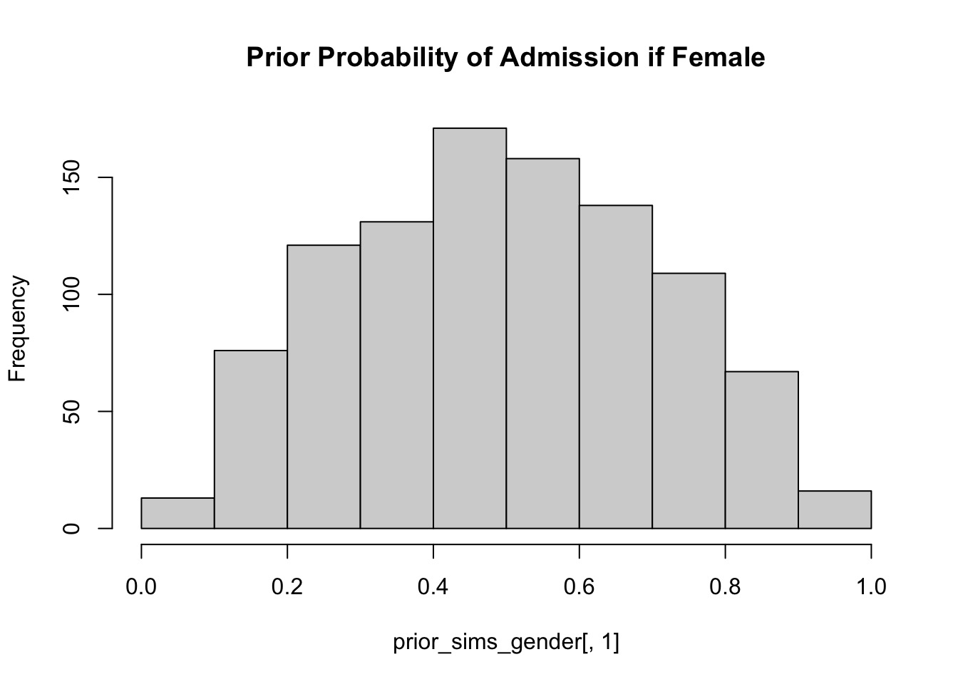
#Let's simulate some priors!
prior_sims <- extract.prior(fit_gender)

# prior sims of gender assuming average no effect of dept - 50:50
prior_sims_gender <- inv_logit(prior_sims$a) 

hist(prior_sims_gender[,1], main = "Prior Probability of Admission if Female")

A Flat Prior in Logit Space Might Not Be Flat!

Let’s try a few SDs to see what works!

prior_frame <- tibble(sd = seq(0.5, 5, 0.5)) %>%
  rowwise() %>%
  mutate(prior_sims = list(rnorm(1e4,0,sd))) %>%
  unnest(prior_sims) %>%
  mutate(prior_sims = inv_logit(prior_sims))

What is our flat prior?

A New Model

mod_gender <- alist(
  #likelihood
  admit ~ dbinom(applications, p),
  
  #Data generating process
  logit(p) <- a[gender] + delta[dept_id],
  
  #priors
  a[gender] ~ dnorm(0,1.5),
  delta[dept_id] ~ dnorm(0,1.5)
)

Fit the Model!

fit_gender <- quap(mod_gender, UCBadmit)

Results… men do slightly worse?

#female = 1, male = 2
precis(fit_gender, depth=2)

               mean        sd       5.5%      94.5%
a[1]     -0.4312203 0.5330873 -1.2831968  0.4207561
a[2]     -0.5279033 0.5322783 -1.3785869  0.3227802
delta[1]  1.1080121 0.5350322  0.2529272  1.9630969
delta[2]  1.0632155 0.5371968  0.2046712  1.9217597
delta[3] -0.1502507 0.5347763 -1.0049265  0.7044252
delta[4] -0.1826522 0.5350901 -1.0378296  0.6725252
delta[5] -0.6246444 0.5378490 -1.4842310  0.2349421
delta[6] -2.1727096 0.5468627 -3.0467019 -1.2987173

Results… men do slightly worse?

What it means

#Women
inv_logit(-0.43)

[1] 0.3941263

#Men
inv_logit(-0.52)

[1] 0.3728522

Relative comparison: Slight Female Advantage? Eh.

samp <- extract.samples(fit_gender)

precis(samp$a[,2] - samp$a[,1], prob=0.8)

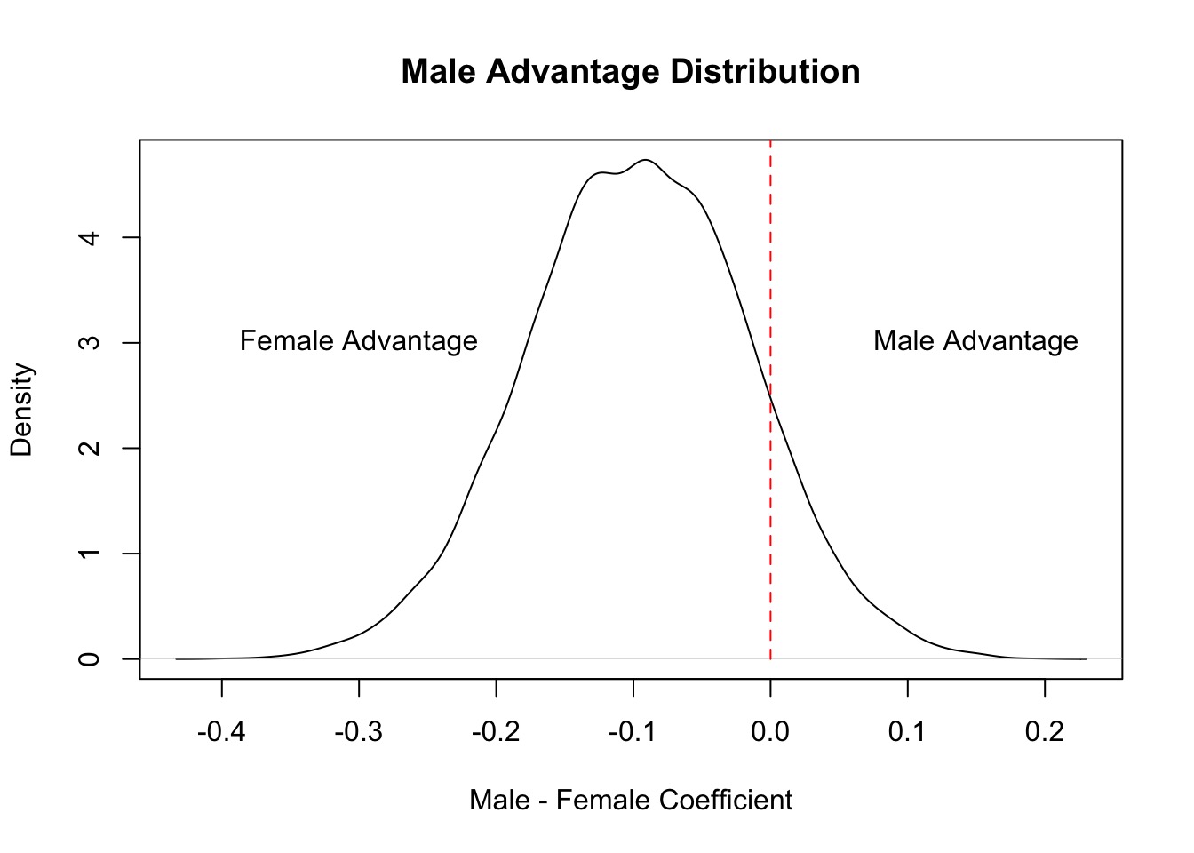
        mean         sd       10%         90%    histogram
 -0.09682634 0.08074047 -0.200614 0.006134635 ▁▁▁▂▅▇▇▅▂▁▁▁

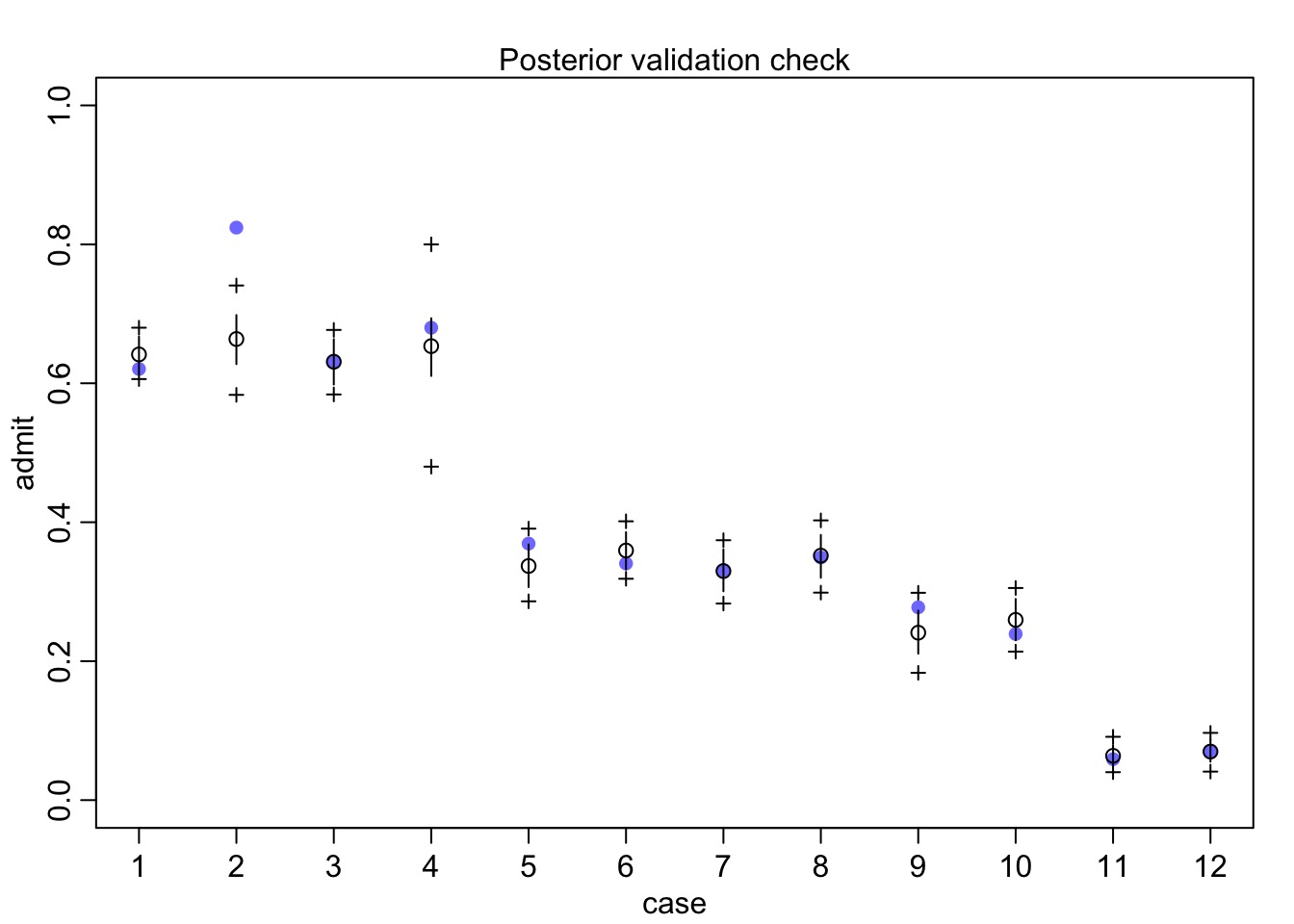
Does our Data Fall in Observations?

Quantile Residuals

qpreds <- add_linpred_draws(UCBadmit, fit_gender) |>
  mutate(.obs = admit/applications) |>
  group_by(dept, applicant.gender) |>
  
  # make an empirical dist of each linpred
  # then get quantile of result
  summarize(dist = list(ecdf(.linpred)),
            .obs = .obs[1],
            q = purrr::map_dbl(.obs[1], dist))

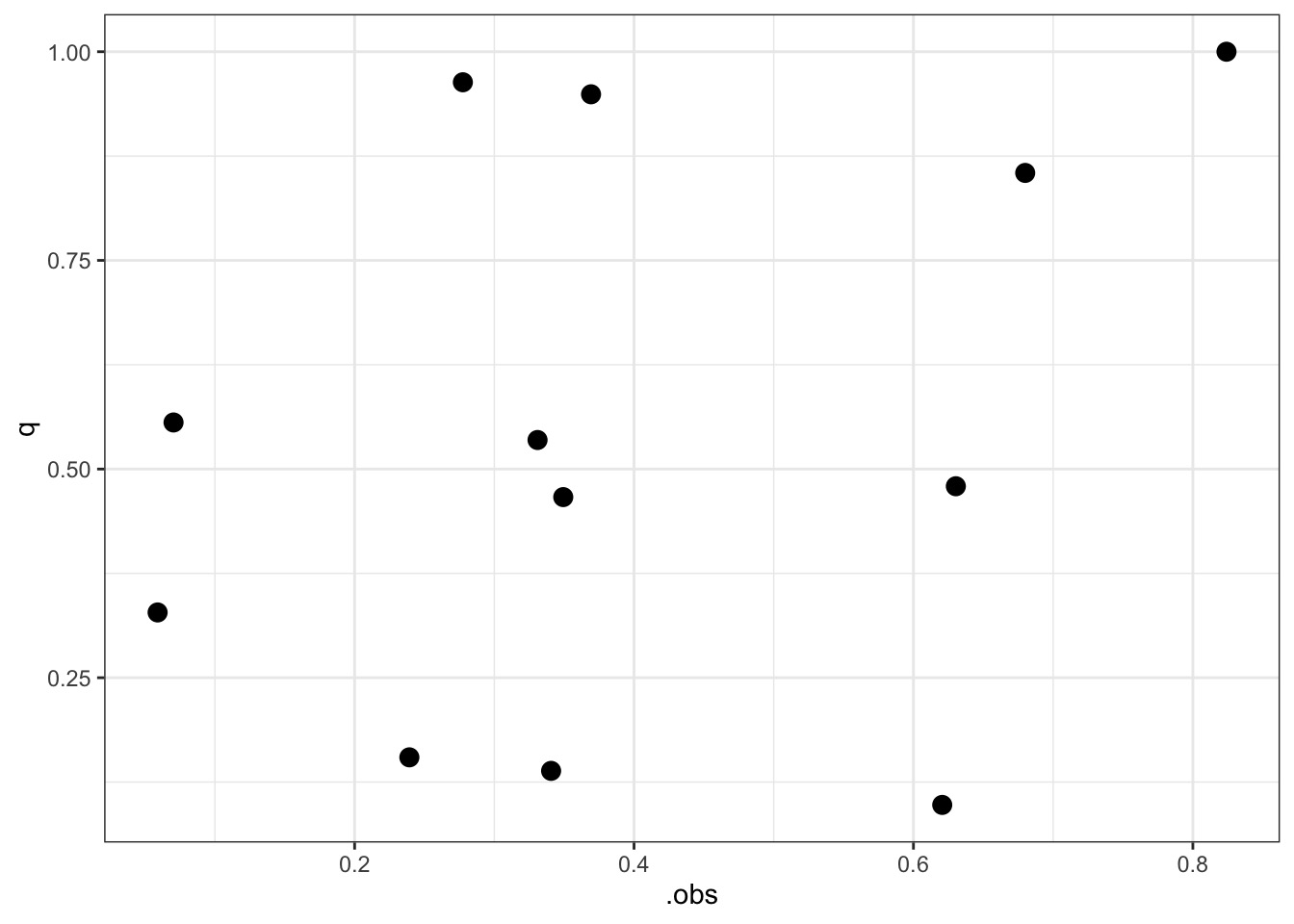
Quantile Residuals and Fits

ggplot(qpreds,
       aes(.obs, q)) +
  geom_point(size = 3)

QQ Unif Check

gap::qqunif(qpreds$q, logscale=FALSE)

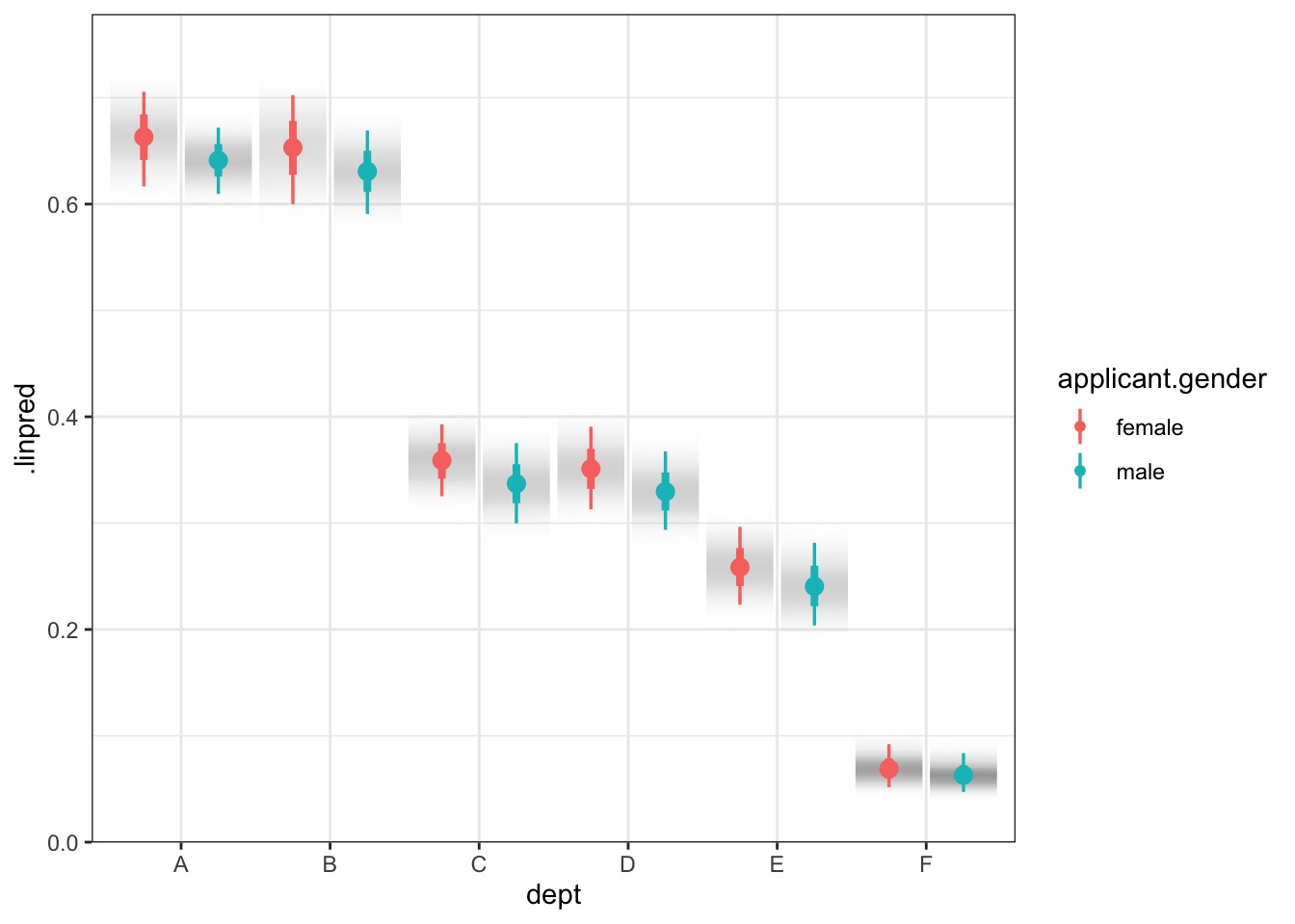
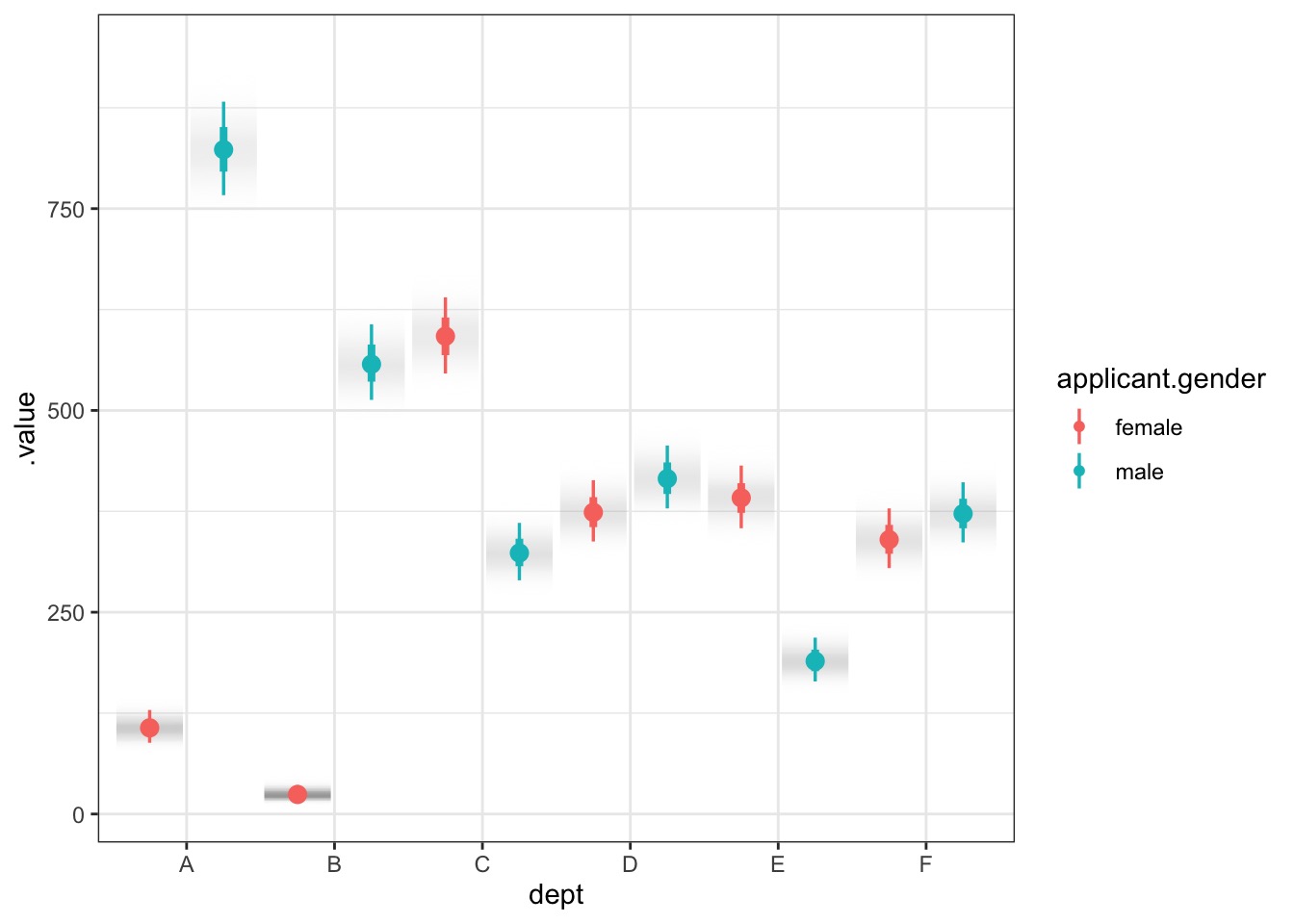
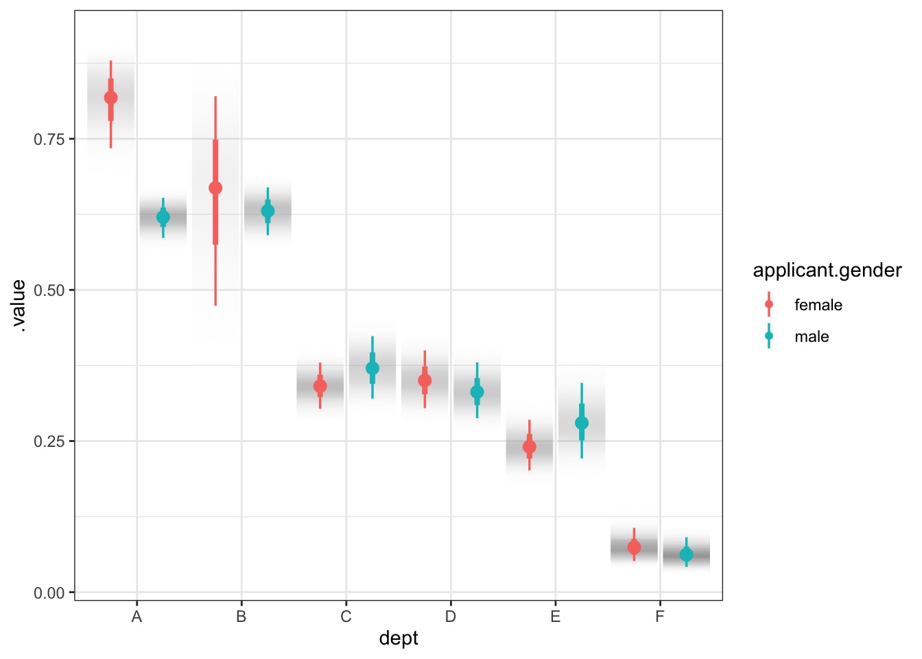
Model Vis with Tidybayes

preds <- add_linpred_draws(UCBadmit, fit_gender)

ggplot(preds, aes(x = dept, y = .linpred,
                  group = applicant.gender, 
                  color = applicant.gender)) +
  stat_gradientinterval(position = "dodge")

Model Vis with Tidybayes

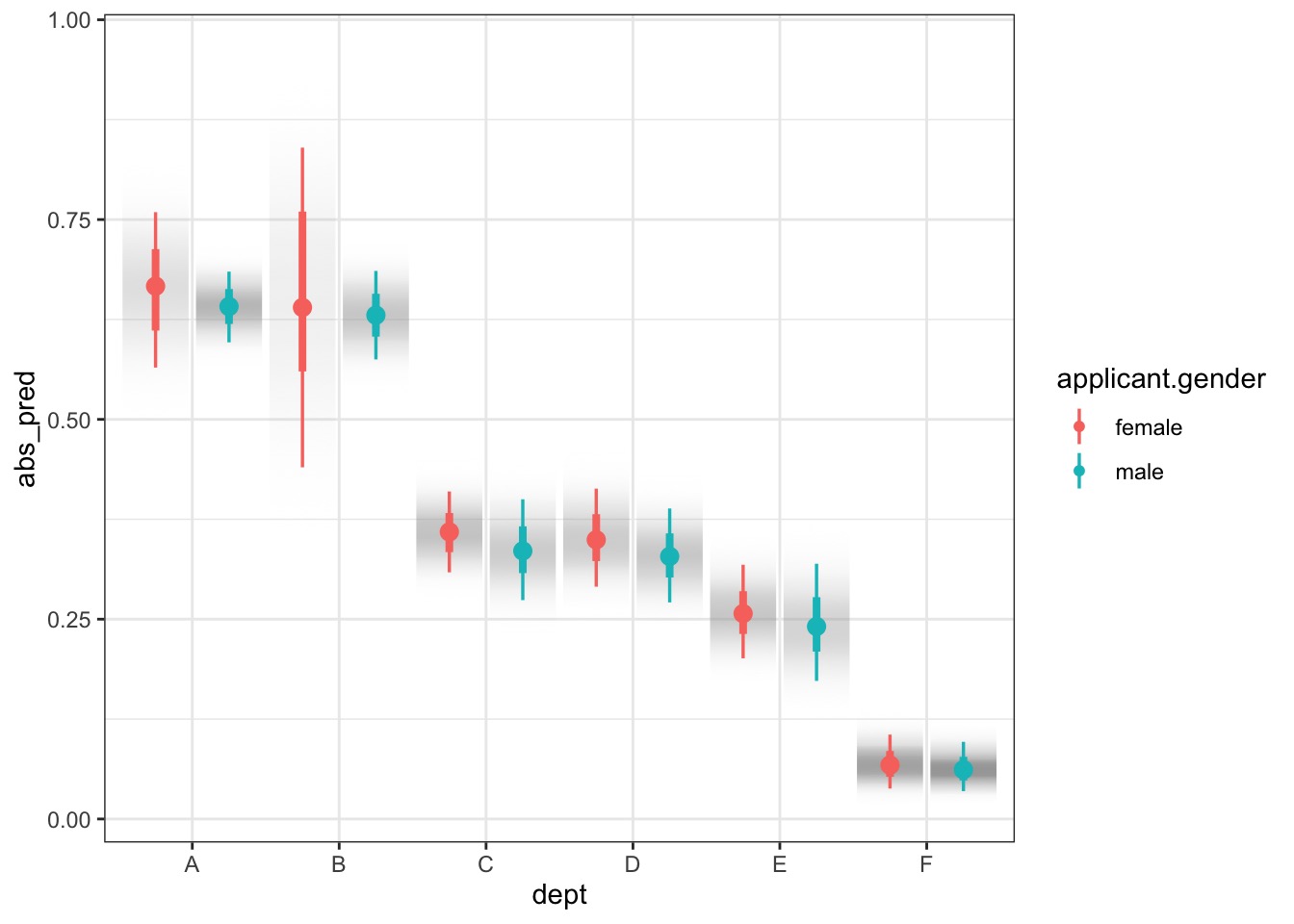
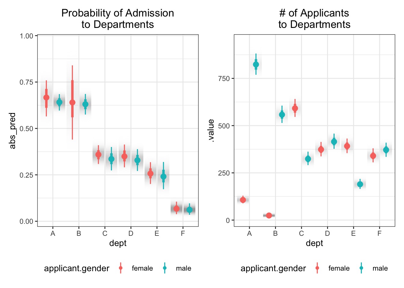
Prediction Intervals and Binomial GLMs

Of course, predictions are 1 or 0 for a straight binomial GLM.
But, more than just coefficient variability is at play
So, we simulate # of successes out of some # of attempts.
Can use this to generate prediction intervals

Prediction Model Vis with Tidybayes

preds_all <- add_predicted_draws(UCBadmit, fit_gender) |>
  mutate(abs_pred = .prediction/applications)

ggplot(preds_all, aes(x = dept, y = abs_pred,
                  group = applicant.gender, 
                  color = applicant.gender)) +
  stat_gradientinterval(position = "dodge")

Prediction Model Vis with Tidybayes

But what about this?

A Generalized Outline

Why use GLMs? An Intro to Entropy
Logistic Regression
Poisson Regression
Poisson -> Multinomial

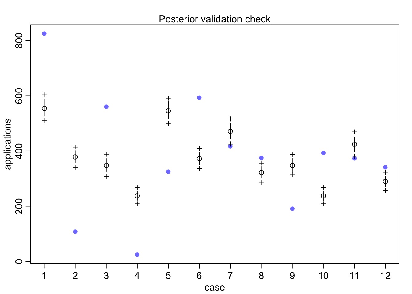
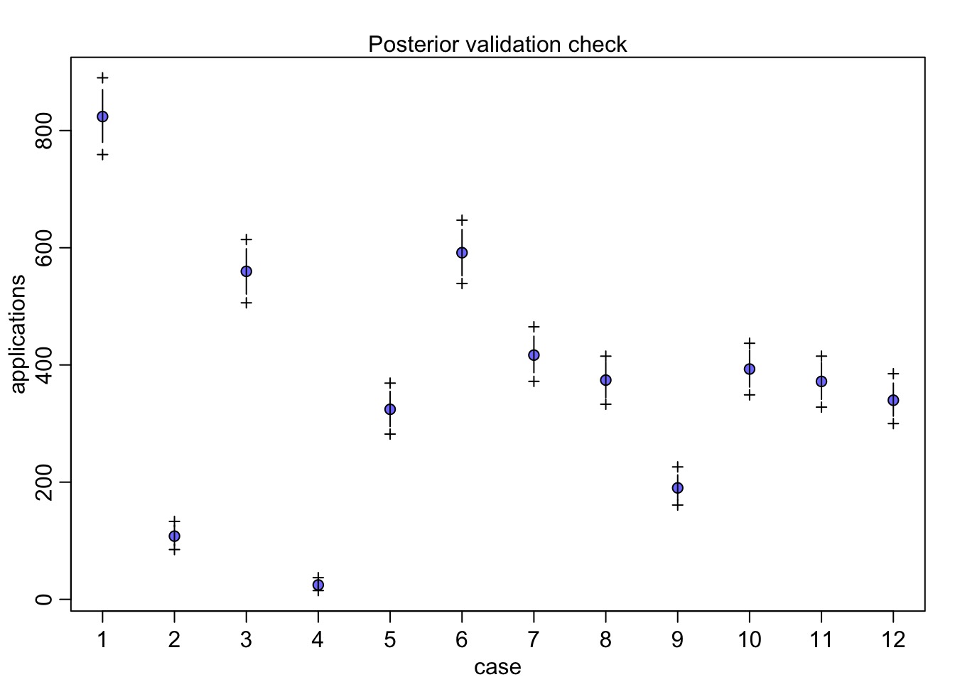
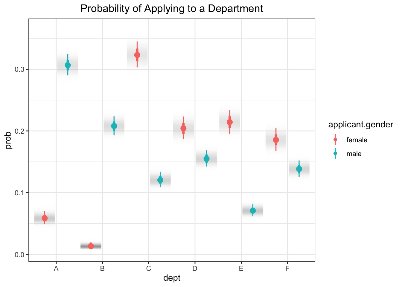
Disparities in Who Applied Where?

Modeling How Gender Influences Application

It could be just different departments get different #s.
It could be gender + department.
It could be differential application by department.

How to determine which non-normal distribution is right for you

Use previous table to determine
Bounded values: binomial, beta, Dirchlet
Counts: Poisson, multinomial, geometric
Distances and durations: Exponential, Gamma (survival or event history)
Monsters: Ranks and ordered categories
Mixtures: Beta-binomial, gamma-Poisson, Zero-inflated processes

Poisson Regression

Likelihood:
\(y_i \sim \mathcal{P}(\lambda)\)

Data Generating Process with identity link
log(\(\lambda_i) = \alpha + \beta_1 x1_i + \beta_2 x2_i + ...\)

Priors:
…

Consider the Gender + Department Model

Likelihood:
\(y_i \sim \mathcal{P}(\lambda)\)

Data Generating Process with identity link
\(log(\lambda_i) = \alpha_{gender} + \beta_{dept}\)

Priors:
\(\alpha_{gender} \sim \mathcal{N}(0,1)\) \(\beta_{dept} \sim \mathcal{N}(0,1)\)

Coded

mod_apply_add <- alist(
  applications ~ dpois(lambda),
  
  log(lambda) <- a[gender] + b[dept_id],
  
  a[gender] ~ dnorm(0,1),
  b[dept_id] ~ dnorm(0,1)
)

fit_apply_add <- quap(mod_apply_add, data = UCBadmit)

Were those reasonable priors?

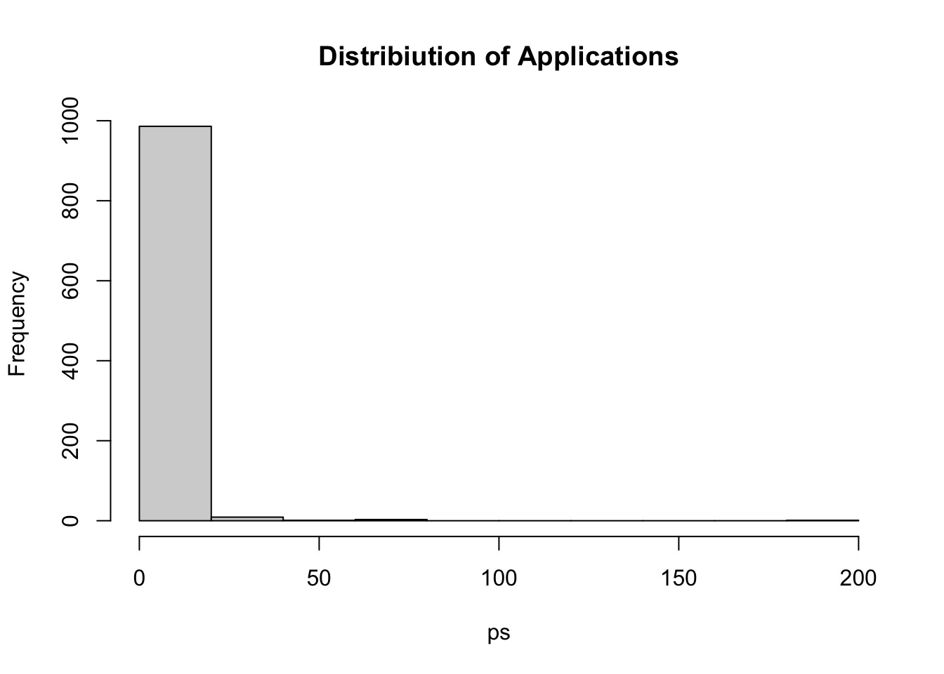
#Let's simulate some priors!
prior_sims_apply <- extract.prior(fit_apply_add)

# What would 1 dept look like for one gender?
ps <- exp(prior_sims_apply$a[,1] + prior_sims_apply$b[,1]) 
 
hist(ps, main = "Distribiution of Applications")

And for real

Up the SD!

Priors at Different SDs

Better Regularizing Priors

mod_apply_add <- alist(
  applications ~ dpois(lambda),
  
  log(lambda) <- a[gender] + b[dept_id],
  
  a[gender] ~ dnorm(0,2),
  b[dept_id] ~ dnorm(0,2)
)

fit_apply_add <- quap(mod_apply_add, data = UCBadmit)

Was this Any Good?

postcheck(fit_apply_add)

What About Gender * Department

UCBadmit <- UCBadmit |>
  mutate(gen_dept = as.numeric(as.factor(paste(gender, dept_id))))

mod_apply <- alist(
  applications ~ dpois(lambda),
  
  log(lambda) <- a[gen_dept],
  
  a[gen_dept] ~ dnorm(0,2)
)

fit_apply <- quap(mod_apply, UCBadmit)

Postcheck

But, More Parameters, so Compare

                   WAIC        SE    dWAIC     dSE      pWAIC weight
fit_apply      110.2433   3.18072    0.000      NA   5.917586      1
fit_apply_add 2221.8544 492.01731 2111.611 515.916 603.643871      0

What does it Mean?

Code

linpred_draws(fit_apply, UCBadmit) |>
  ggplot(
       aes(x = dept, y = .value,
           group = applicant.gender, 
           color = applicant.gender)) +
  stat_gradientinterval(position = "dodge")

It’s an Indirect Effect of Gender

A Generalized Outline

Why use GLMs? An Intro to Entropy
Logistic Regression
Poisson Regression
[Poisson = Multinomial]]{style=“color:red”}

Lingering Questions

Well, maybe admission bias differs by departments?
Can we turn our application results into probabilities to calculate direct, indirect, and total effects?

Does Bias Differ by Department?

                 WAIC        SE    dWAIC      dSE    pWAIC       weight
fit_gen_int  90.21511  3.396592  0.00000       NA 6.457929 0.9998486738
fit_gender  107.80696 15.647798 17.59184 16.52952 9.044645 0.0001513262

Department A is Biased Towards Women - Although Fewer Apply

Q2: How to Turn Poisson Model into Probabilities

Normally we’d use a multinomial to get probabilities of multiple classes. \[X \sim Mult(n, \pi)\]
BUT - a poisson with categories can turn into a multinomial!

Poisson to Multinomial

\[X \sim Mult(n, \pi)\]

If \[X_1 \sim P(\lambda_1)\] \[X_2 \sim P(\lambda_2)\] … \[X_k \sim P(\lambda_k)\]

then n = \(X_1 + X_2 +....X_k\) where \(\pi=(\pi_1,\ldots,\pi_k)\)

So: \[\pi_j=\dfrac{\lambda_j}{\lambda_1+\cdots+\lambda_k}\]

Using our Model for Estimating Pi

We Can Use our Predictions as Lambda

probs <- linpred_draws(fit_apply, UCBadmit) |>
  group_by(.draw, applicant.gender) |>
  mutate(prob = .value / sum(.value)) |>
  ungroup()

Big Disparities in Where Different Genders Apply

Calculating the Probabilities of Getting Into Dept A as a Woman

Direct Probability of Admission if a Woman:

[1] 0.8152725

Probability of Applying to A if a Woman:

[1] 0.05875285

0.06 * 0.81 = 0.0486