Bayesian Linear Regression

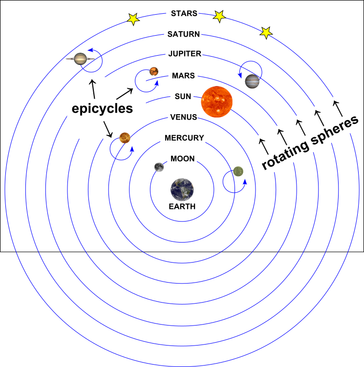
A Ptolemeic Model of the Universe

Why a Normal Error Distribution

• Good descriptor of sum of many small errors
  
• True for many different distributions

A Normal Error Distribution and Many Small Errors

par(mfrow=c(1,2))
set.seed(100)
z <- replicate(100, cumsum(rnorm(100)))
matplot(z, type="l", col="grey")
simplehist(replicate(1000, sum(rnorm(100))))
par(mfrow=c(1,1))

Or in Continuous Space

set.seed(2019)
samps <- replicate(1e5, sum(1 + runif(100,0,1)))
plot(density(samps))

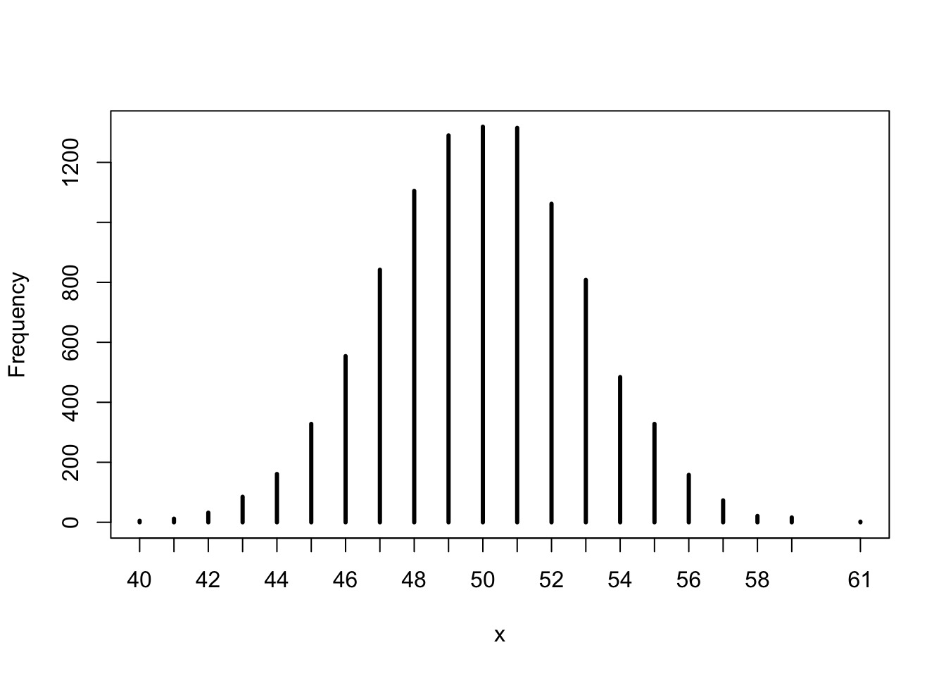
Gaussian Behavior from Many Distributions

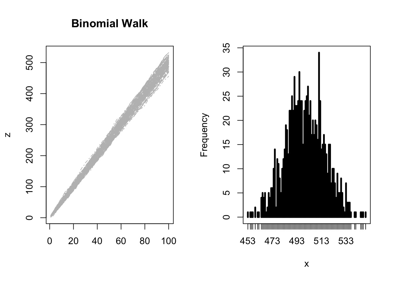
Code

par(mfrow=c(1,2))
set.seed(100)
z <- replicate(100, cumsum(rbinom(100,10,.5)))
matplot(z, type="l", col="grey", main="Binomial Walk")
simplehist(replicate(1000, sum(rbinom(100,10,.5))))
par(mfrow=c(1,1))

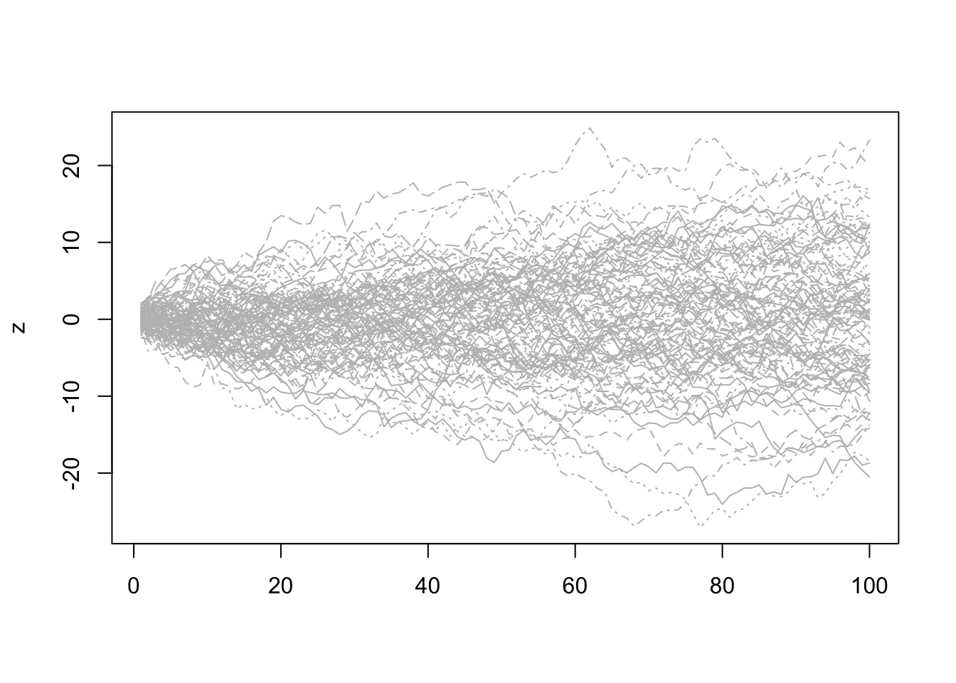
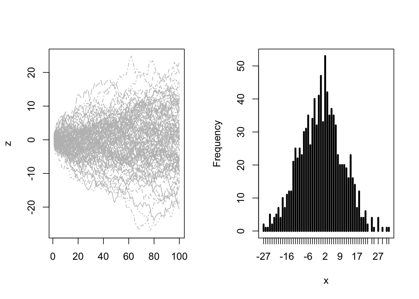
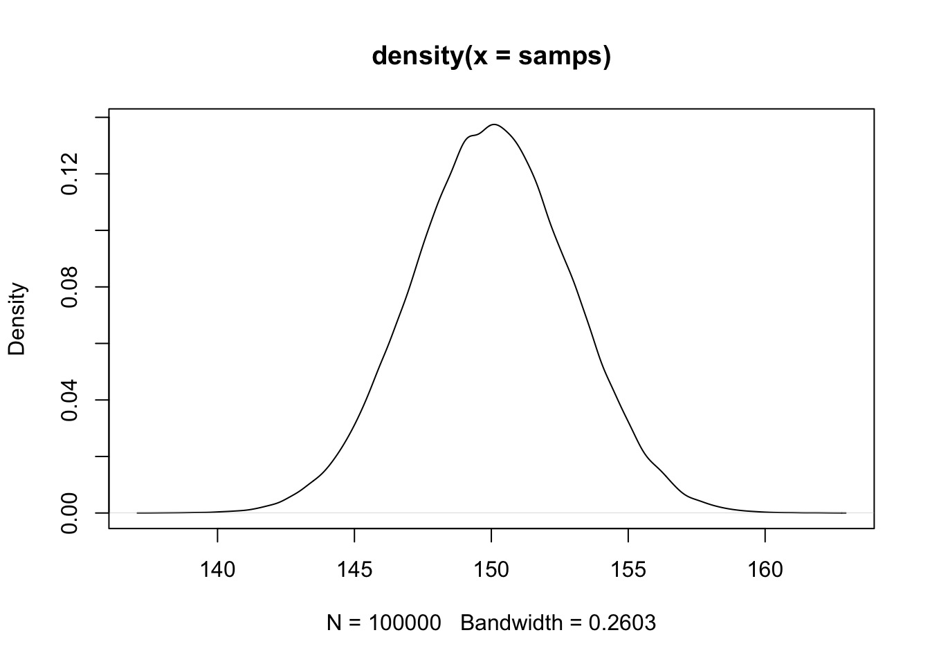
Try it: the Central Limit Theorem

library(rethinking)
simplehist(replicate(1e4, sum(rbeta(100,1,1))))

But, Is the World an Accumulation of Small Errors?

Linear Regression: A Simple Statistical Golem

• Describes association between predictor and response
  
• Response is additive combination of predictor(s)
  
• Constant variance

Why should we be wary of linear regression?

• Approximate
  
• Not mechanistic
  
• Often deployed without thought
  
• But, often very accurate

So, how do we build models?

1. Identify response

2. Determine likelihood (distribution of error of response)

3. Write equation(s) describing generation of predicted values

4. Assign priors to parameters

Our Previous Model

Likelihood:
\(w \sim Binomial(6, size=9, prob = prob)\)

Prior:
\(prob \sim Uniform(0,1)\)

A Normal/Gaussian Model

Likelihood:
\(y_i \sim Normal( \mu, \sigma)\)

Prior:
\(\mu \sim Normal(0,1000)\)
\(\sigma \sim U(0,50)\)

A Model of a Mean Height from the !Kung San

data(Howell1)
Howell1_Adult <- Howell1 %>% 
  filter(age >= 18)

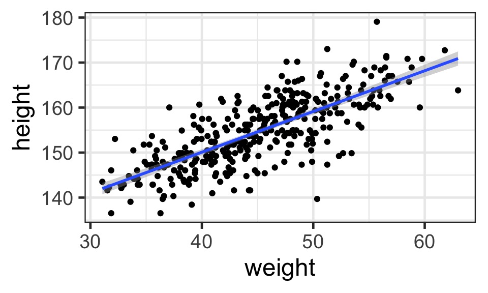
What does the data look like?

precis(Howell1_Adult)

            mean         sd     5.5%     94.5%       histogram
height 154.59709  7.7423321 142.8750 167.00500       ▁▃▇▇▅▇▂▁▁
weight  44.99049  6.4567081  35.1375  55.76588         ▁▅▇▇▃▂▁
age     41.13849 15.9678551  20.0000  70.00000 ▂▅▇▅▃▇▃▃▂▂▂▁▁▁▁
male     0.46875  0.4997328   0.0000   1.00000      ▇▁▁▁▁▁▁▁▁▇

Our Model of Height

Likelihood:
\(h_i \sim Normal( \mu, \sigma)\)

Prior:
\(\mu \sim Normal(187, 20)\) My Height
\(\sigma \sim U(0,50)\) Wide range of possibilities

Priors

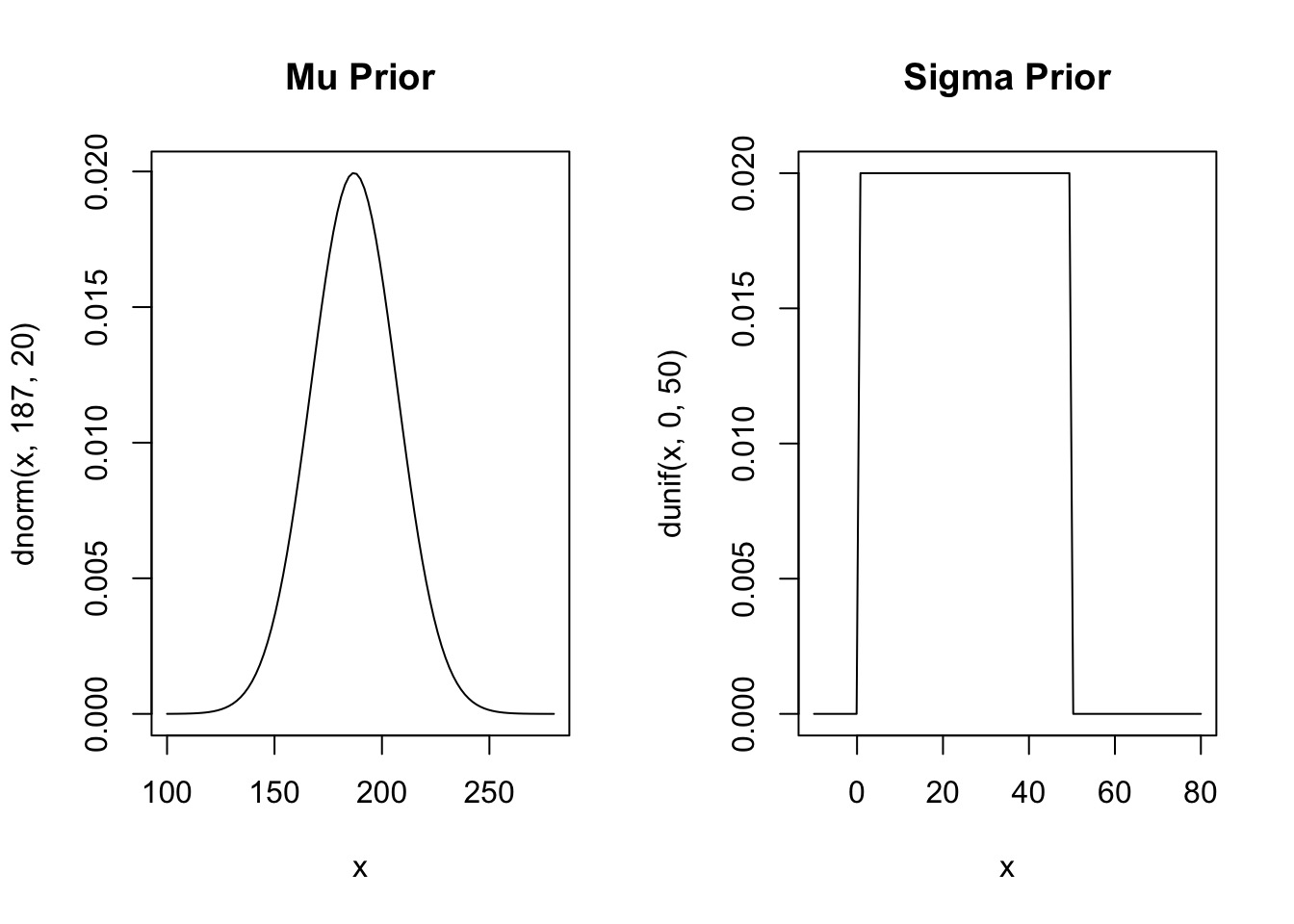
Prior Predictive Simulation

• Are your priors any good?

• Simulate from them to generate fake data

• Does simulated data look realistic?

• Does simulated data at least fall in the range of your data?

Example:

Prior:
\(\mu \sim \mathcal{N}(187, 20)\) My Height
\(\sigma \sim \mathcal{U}(0,50)\) Wide range of possibilities

set.seed(2019)
n <- 1e4
prior_m <- rnorm(n, 187, 20)
prior_s <- runif(n, 0, 50)
prior_h <- rnorm(n, prior_m, prior_s)

Reasonable? Giants and Negative People?

Prior:
\(\mu \sim \mathcal{N}(187, 20)\) My Height
\(\sigma \sim \mathcal{U}(0,50)\) Wide range of possibilities

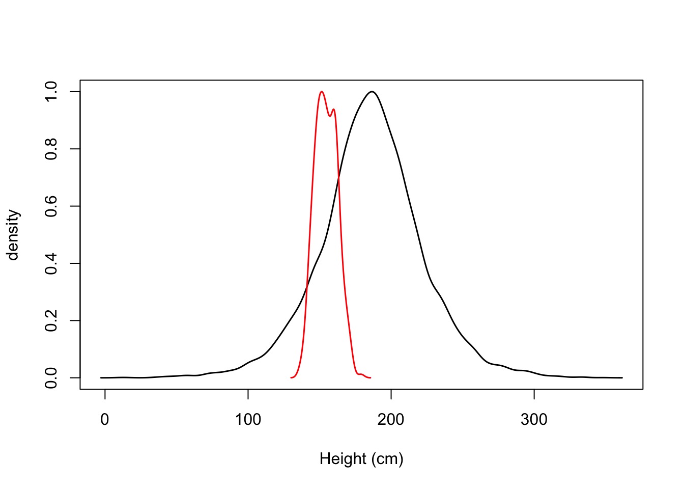
OK, I’m Tall, And Not Even In the Data, So….

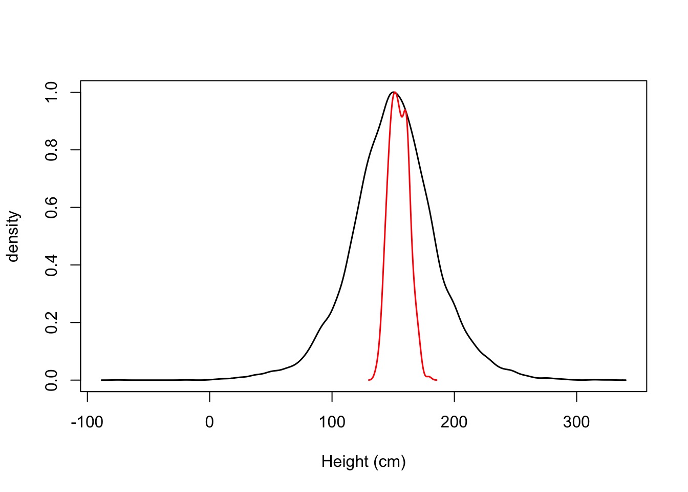
Prior:
\(\mu \sim \mathcal{N}(150, 20)\) Something More Reasonable
\(\sigma \sim \mathcal{U}(0,50)\) Wide range of possibilities

Grid Sampling

# Make the grid
grid <- tidyr::crossing(mu = seq(140, 160, length.out=200),
                 sigma = seq(4, 9, length.out=200)) |>

#Calculate the log-likelihoods for each row  
  group_by(1:n()) %>%
  mutate(log_lik = sum(dnorm(Howell1_Adult$height, mu, sigma, log=TRUE))) %>%
  ungroup() %>%

# Use these and our posteriors to get the numerator
# of Bayes theorem
  mutate(numerator = log_lik + 
           dnorm(mu, 150, 20, log=TRUE) +
           dunif(sigma, 0,50, log=TRUE)) |>

#Now calculate the posterior (approximate)  
  mutate(posterior = exp(numerator - max(numerator)))

Posterior

ggplot(grid,
       aes(x = mu, y = sigma, alpha = posterior, color = posterior)) +
  geom_point() +
  scale_alpha_continuous(range=c(0,1)) +
  scale_color_viridis_c()

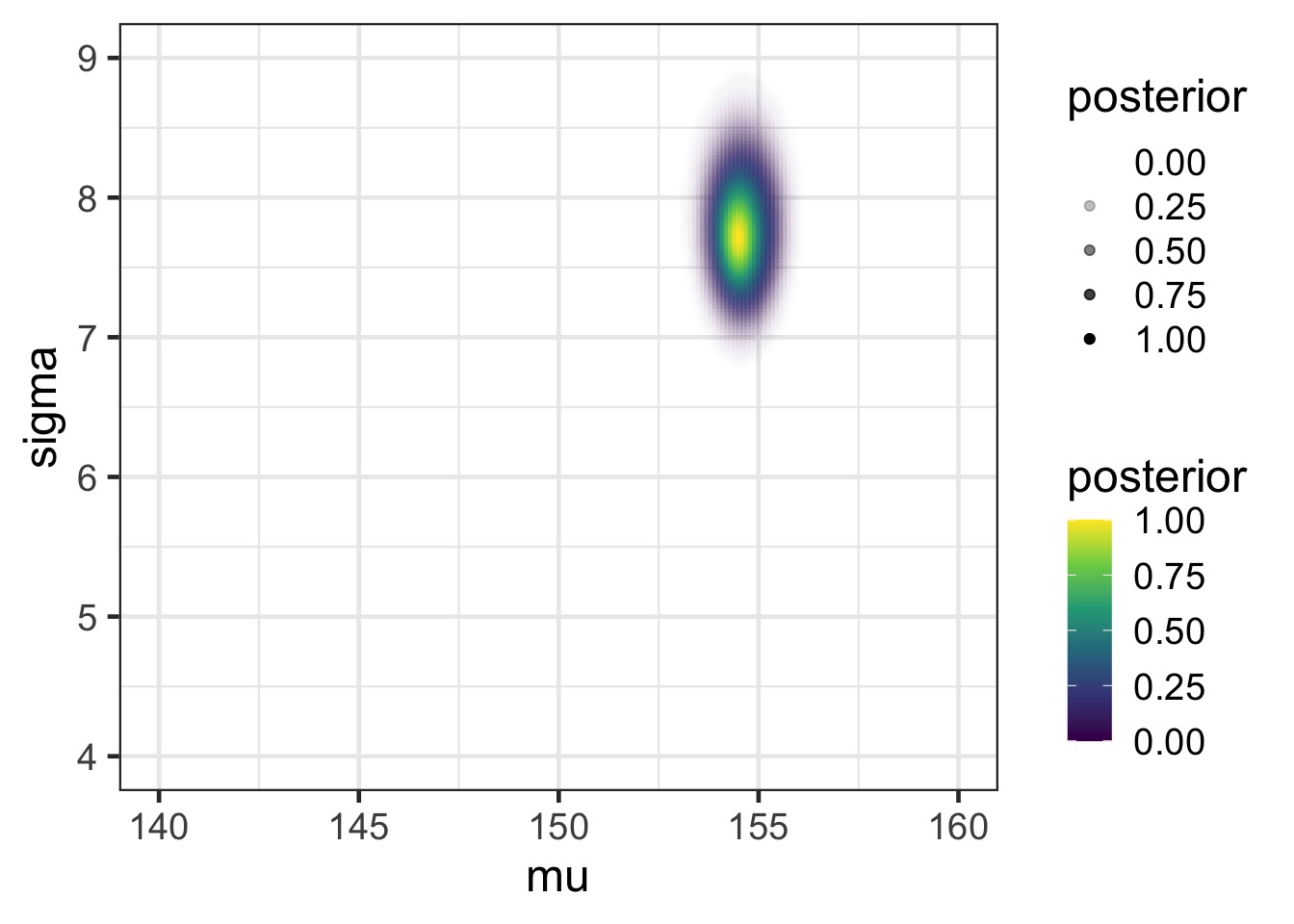
Posterior from a Sample of the Grid

samp <- grid[sample(1:nrow(grid), size=1e4, replace=TRUE, prob=grid$posterior),1:2]
ggplot(samp, aes(x = mu, y = sigma)) +
  geom_point(alpha = 0.3, color = "blue")

Or, let’s Reconceptualize With a Model

Likelihood:
\(h_i \sim \mathcal{N}( \mu, \sigma)\)    height ~ dnorm(mu, sigma)

Prior:
\(\mu \sim \mathcal{N}(150, 20)\)    mu ~ dnorm(150, 200)
\(\sigma \sim U(0,50)\)    sigma ~ dunif(0,50)

Building Models using rethinking: The alist Object

mean_mod <- alist(
  #likelihood
  height ~ dnorm(mu, sigma),
  
...

Building Models using rethinking: The alist Object

mean_mod <- alist(
  #likelihood
  height ~ dnorm(mu, sigma),
  
  #priors
  mu ~ dnorm(150, 20),
  sigma ~ dunif(0,50)
)

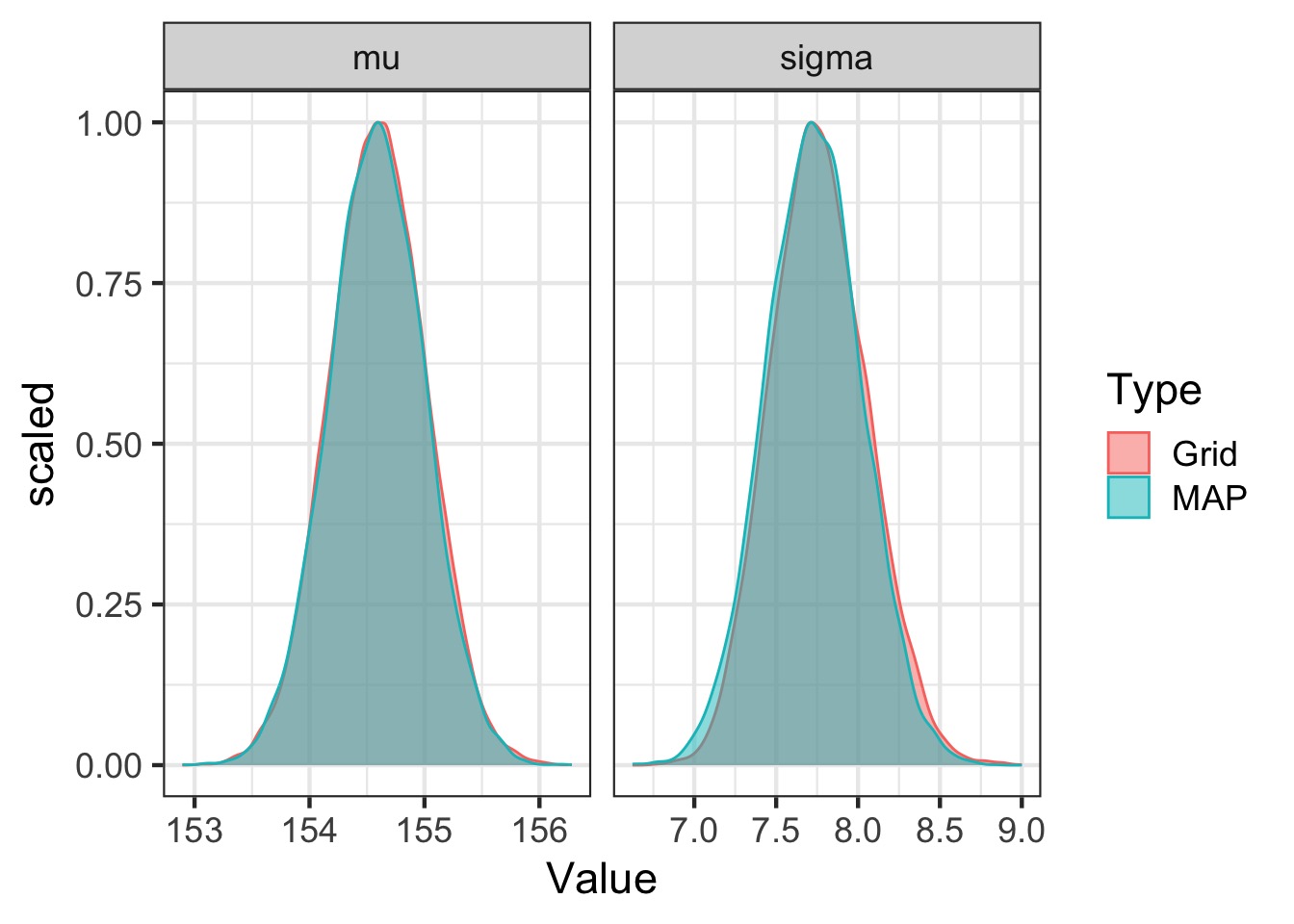
Feed the Model to Maximum A Posterior Approximation

mean_fit <- quap(mean_mod,
                data = Howell1_Adult)

• Uses optimization algorithms
  
• Same algorithms as likelihood

Compare map to grid

Adding a Predictor

1. Identify response (height)

2. Determine likelihood (distribution of error of response)

3. Write equation(s) describing generation of predicted values

   • Weight predicts height

4. Assign priors to parameters

   • Check priors with simulation

The Mean Changes with predictor: A Linear Model!

Likelihood:
\(h_i \sim \mathcal{N}(\mu_i, \sigma)\)

Data Generating Process
\(\mu_i = \alpha + \beta (x_i - \bar{x_i})\)

Prior:
\(\alpha \sim \mathcal{N}(150, 20)\)   Previous Mean
\(\beta \sim \mathcal{N}(0, 10)\)   Weakly Informative
\(\sigma \sim \mathcal{U}(0,50)\)  Wide range of possibilities

Let’s have the Centering Talk. Why?

Let’s Check our Priors! But Over what range?

range(Howell1_Adult$weight)

[1] 31.07105 62.99259

So, ± 15

When in doubt, simulate it out!

set.seed(2019)
n <- 100

# a data frame of priors
sim_priors_df <- data.frame(a = rnorm(n, 150, 20),
                        b = rnorm(n, 0, 10))


# geom_abline to make lines
prior_plot <- ggplot(data = sim_priors_df) +
    geom_abline(mapping = aes(slope = b, intercept = a)) +
  xlim(c(-15,15)) + ylim(c(-100, 500)) +
  xlab("Weight - Mean Weight") + ylab("Height (cm)") 

Giants and Negative Humans?

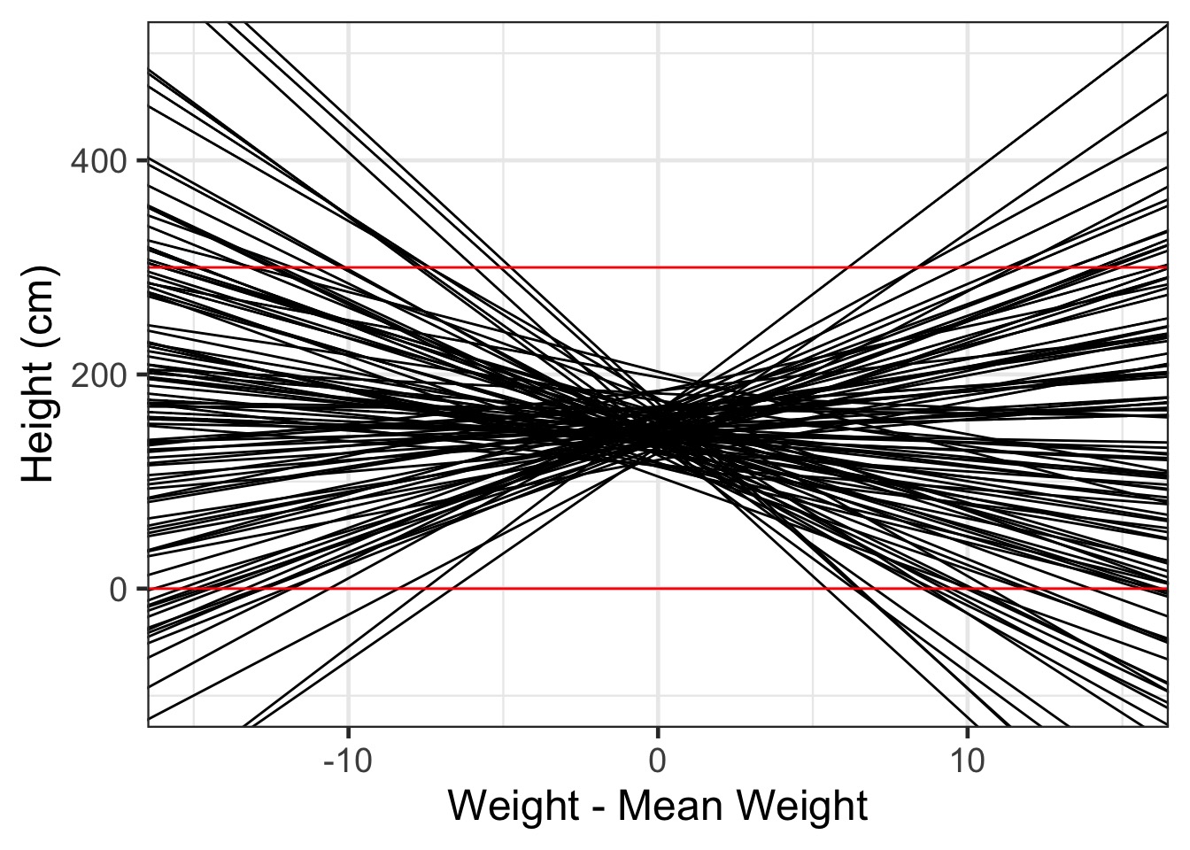
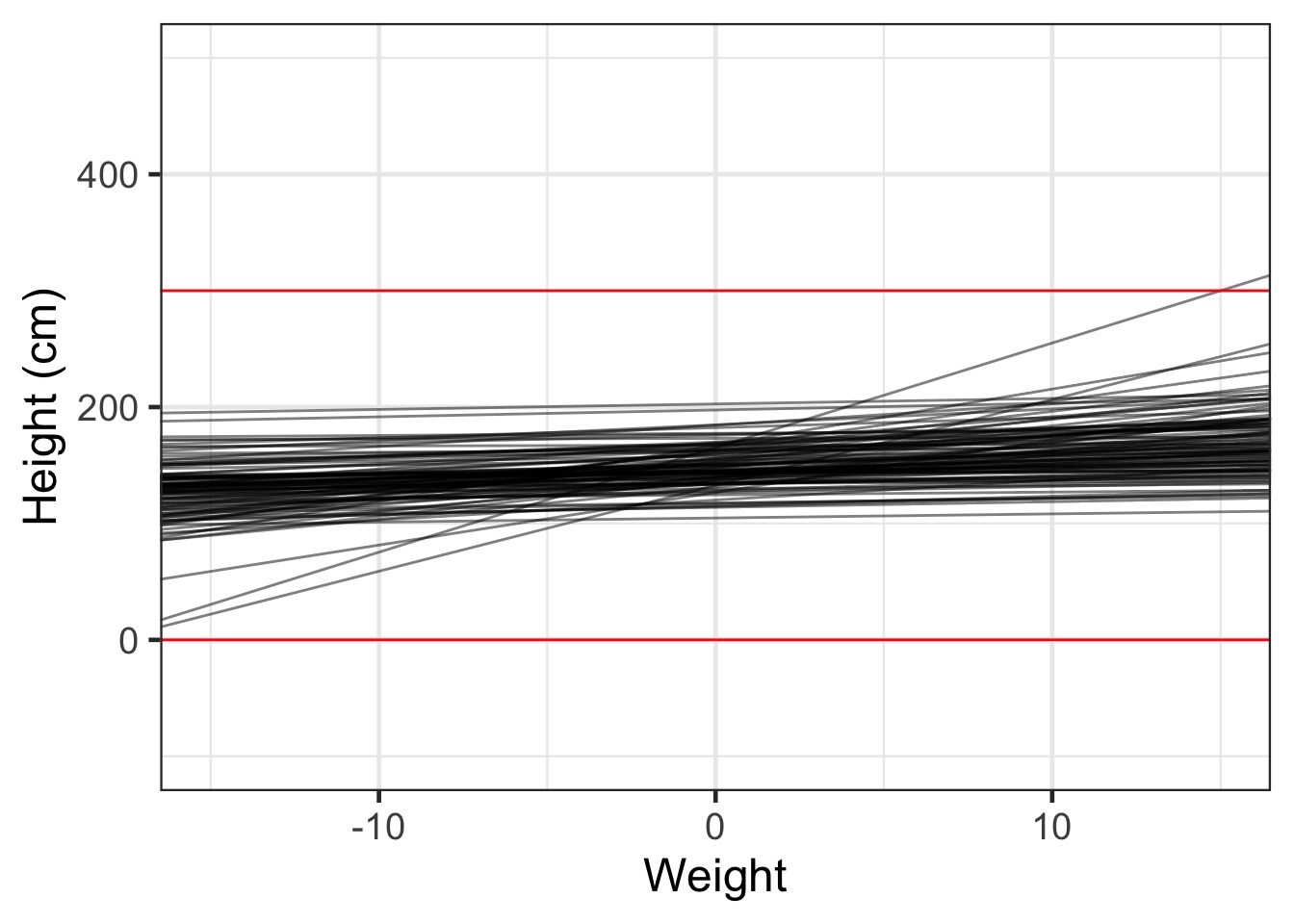
Rethinking our Priors!

Try a log-normal to guaruntee a positive value!

rnorm(10, 0, 10)

 [1]   7.208450  -3.946306   9.826626 -14.043020   8.002034  -7.507425
 [7] -17.869624   6.412382  -7.564241   6.945962

rlnorm(10, 0, 1)

 [1] 2.8380974 0.8909155 0.2886832 0.1285018 1.1239655 1.4806061 0.8809009
 [8] 0.7026157 3.6836816 0.4159838

The Log Normal

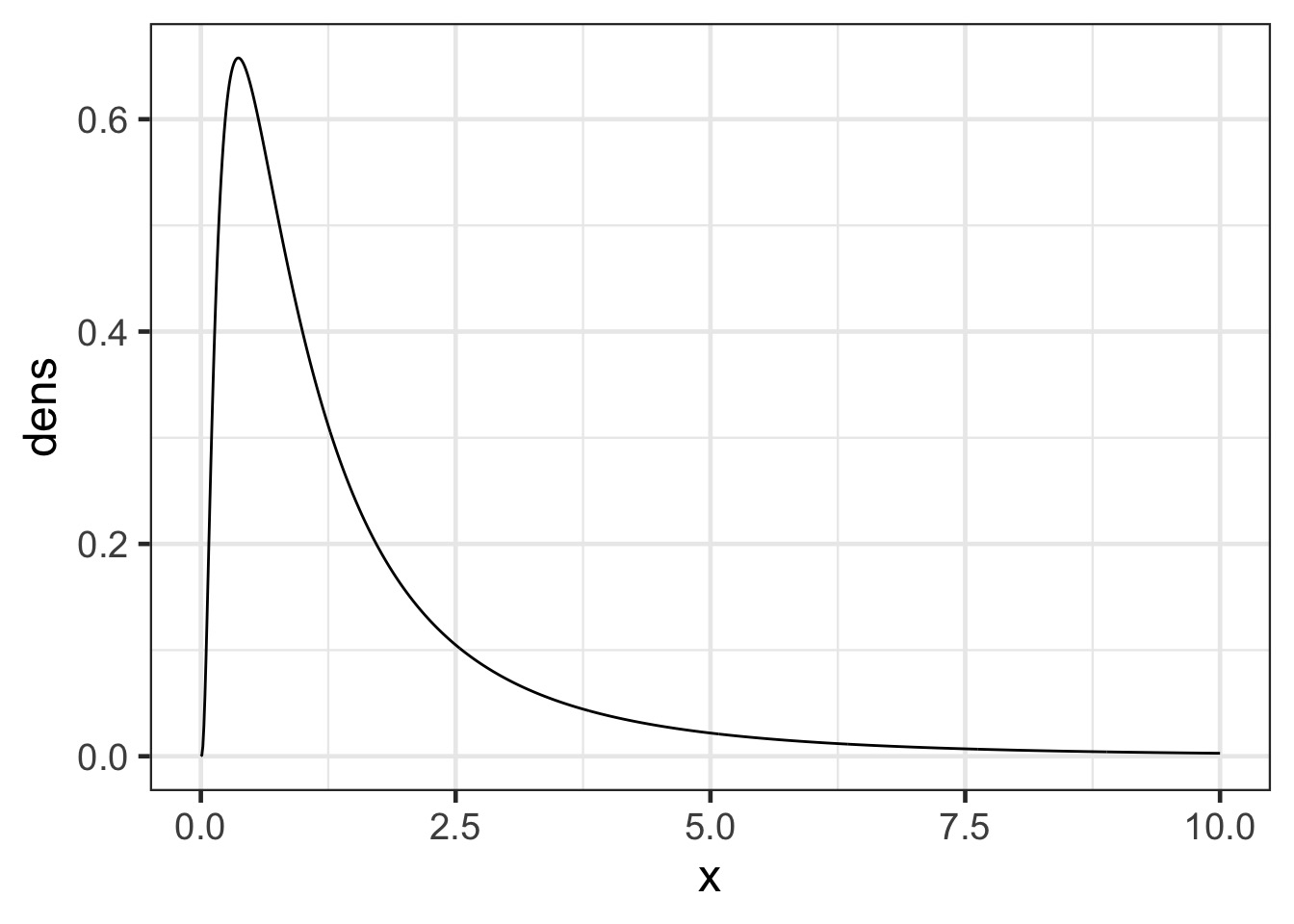
Simulate it out!

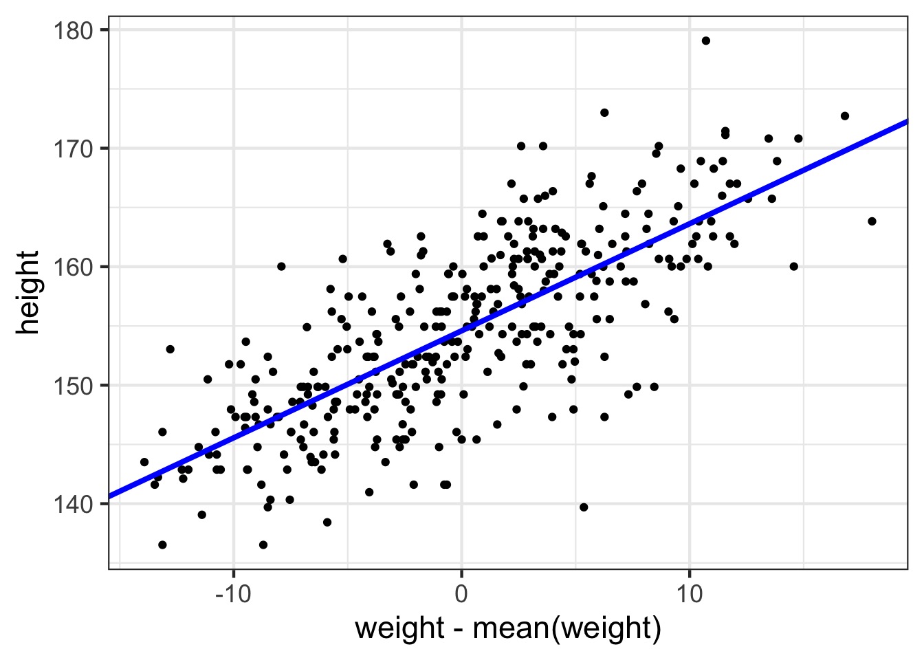
Our Linear Model

weight_mod <- alist(
  #likelihood
  height ~ dnorm(mu, sigma),
  
  #Data generating process
  mu <- alpha + beta * (weight-mean(weight)),
  
  #priors
  alpha ~ dnorm(150, 20),
  beta ~ dlnorm(0, 1),
  sigma ~ dunif(0,50)
)

weight_fit <- quap(weight_mod,
                data = Howell1_Adult)

The Coefficients

precis(weight_fit)

             mean         sd      5.5%       94.5%
alpha 154.5962531 0.27030757 154.16425 155.0282568
beta    0.9032821 0.04192365   0.83628   0.9702841
sigma   5.0718827 0.19115492   4.76638   5.3773852

See the fit

base_plot <- ggplot(data=Howell1_Adult,
                    mapping=aes(x=weight-mean(weight), y=height)) +
  geom_point() +
  theme_bw(base_size=17)

base_plot+
  geom_abline(slope=coef(weight_fit)[2], 
              intercept=coef(weight_fit)[1],
              color="blue", lwd=1.4)

The fit

So, what do we do with a fit model?

1. Evaluate model assumptions

2. Evaluate model estimates and meaning

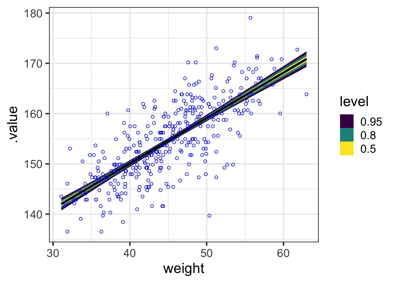
3. Assess uncertainty in fit

4. Assess uncertainty in prediction

Sampling From Models with tidybayes

library(tidybayes)
library(tidybayes.rethinking)

• We will use this as tidybayes is great for many Bayesian Packages.

• Obeys a common tidy formatting

linpred_draws() for Link Predictions

weight_samps <- 
  linpred_draws(weight_fit, 
                newdata = Howell1_Adult, 
                ndraws = 1000)

head(weight_samps)

# A tibble: 6 × 7
# Groups:   height, weight, age, male, .row [1]
  height weight   age  male  .row .draw .value
   <dbl>  <dbl> <dbl> <int> <int> <int>  <dbl>
1   152.   47.8    63     1     1     1   157.
2   152.   47.8    63     1     1     2   157.
3   152.   47.8    63     1     1     3   158.
4   152.   47.8    63     1     1     4   157.
5   152.   47.8    63     1     1     5   157.
6   152.   47.8    63     1     1     6   157.

Get Residuals and a Summarized Frame

weight_samps <- weight_samps |>
  mutate(.residuals = height - .value)

weight_samps_summarized <- weight_samps |>
  group_by(height, weight, .row) |>
  summarize(
    .mean_resid = mean(.residuals),
    .mean = mean(.value),
    .lower_pi = PI(.value)[1],
    .upper_pi = PI(.value)[2],
    .groups = "drop"
  )

Check Posterior Against Data

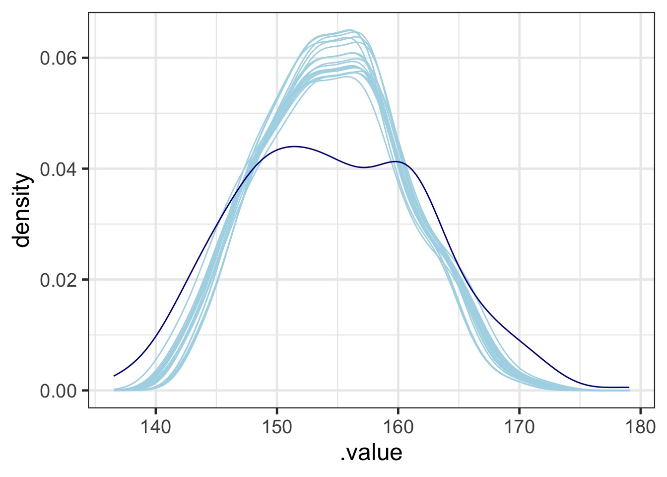
Code for PP Check

ggplot() +
  geom_density(data = weight_samps |> filter(.draw < 20),
               aes(group = .draw, x = .value),
               alpha = 0.02, color = "lightblue") +
  geom_density(data = Howell1_Adult, aes(x = height), color = "darkblue")

QQ, etc…

qqnorm(weight_samps_summarized$.mean_resid)
qqline(weight_samps_summarized$.mean_resid)

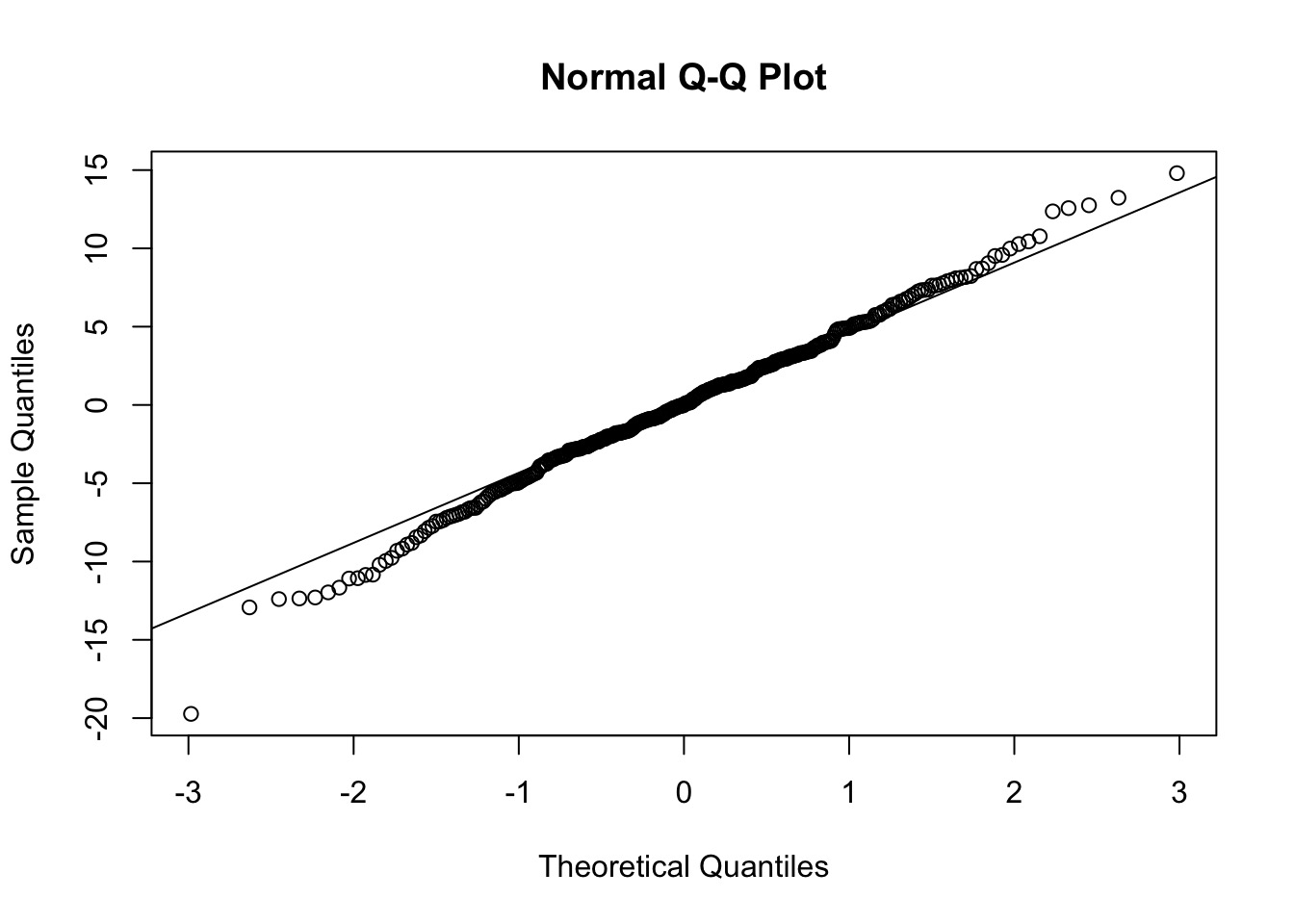
Fit-Residual

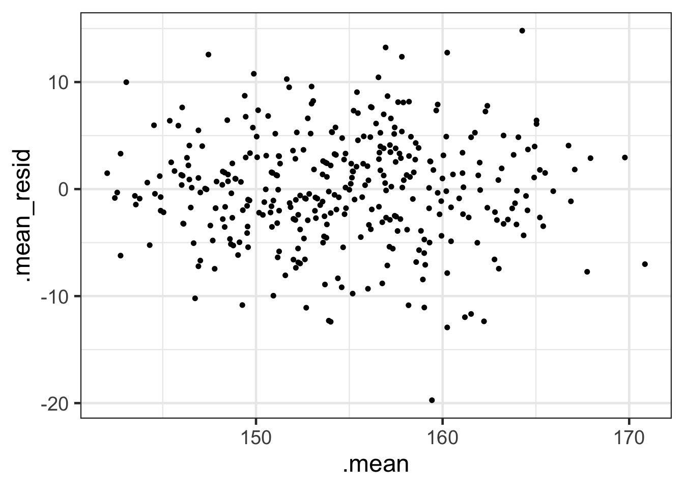
Code

ggplot(weight_samps_summarized, 
       aes(x=.mean_resid, y=.mean)) +
  geom_point(size=1.3)  +
  coord_flip()

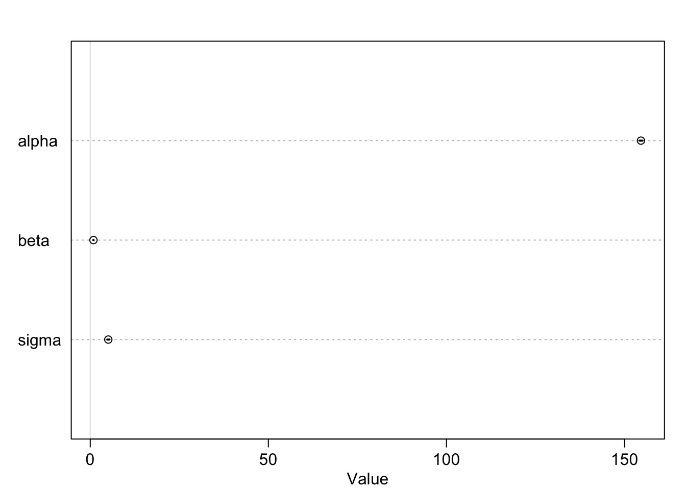
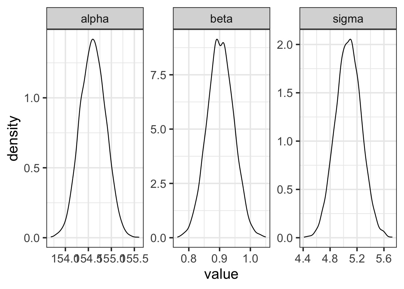
Model Results

precis(weight_fit, cor=TRUE)

             mean         sd      5.5%       94.5%
alpha 154.5962531 0.27030757 154.16425 155.0282568
beta    0.9032821 0.04192365   0.83628   0.9702841
sigma   5.0718827 0.19115492   4.76638   5.3773852

• Are these meaningful?

• Should you standardize predictors for a meaningful intercept?

• Is this the right interval?

Model Results

Sampling from the Posterior Distribution

post <- tidy_draws(weight_fit)

head(post)

# A tibble: 6 × 6
  .chain .iteration .draw alpha  beta sigma
   <int>      <int> <int> <dbl> <dbl> <dbl>
1     NA         NA     1  154. 0.915  5.12
2     NA         NA     2  154. 0.918  5.06
3     NA         NA     3  155. 0.913  4.82
4     NA         NA     4  154. 0.842  4.67
5     NA         NA     5  155. 0.896  4.93
6     NA         NA     6  155. 0.819  4.92

Posteriors!

Code

tidyr::pivot_longer(post, alpha:sigma) |>
  ggplot(aes(x = value)) +
  geom_density() +
  facet_wrap(vars(name), scale = "free")

Relationships?

ggplot(data = post, aes(x = alpha, y = beta)) +
  geom_point(alpha = 0.2, color = "blue")

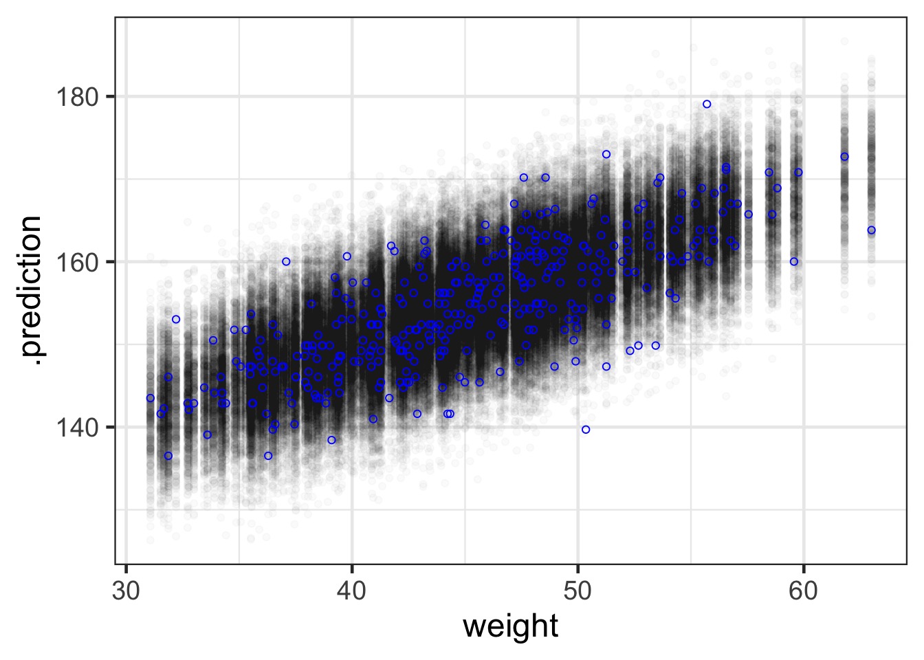
How Well Have we Fit the Data? Use Samples of Data

ggplot() +
  
  #simulated fits from the posterior
  geom_line(data=weight_samps |> filter(.draw < 500), 
              mapping=aes(x = weight, 
                          y = .value, 
                          group = .draw), alpha=0.02) +
  
  #the data
  geom_point(data=Howell1_Adult, 
             mapping=aes(x=weight, y=height), pch=1, color = "blue") 

How Well Have we Fit the Data?

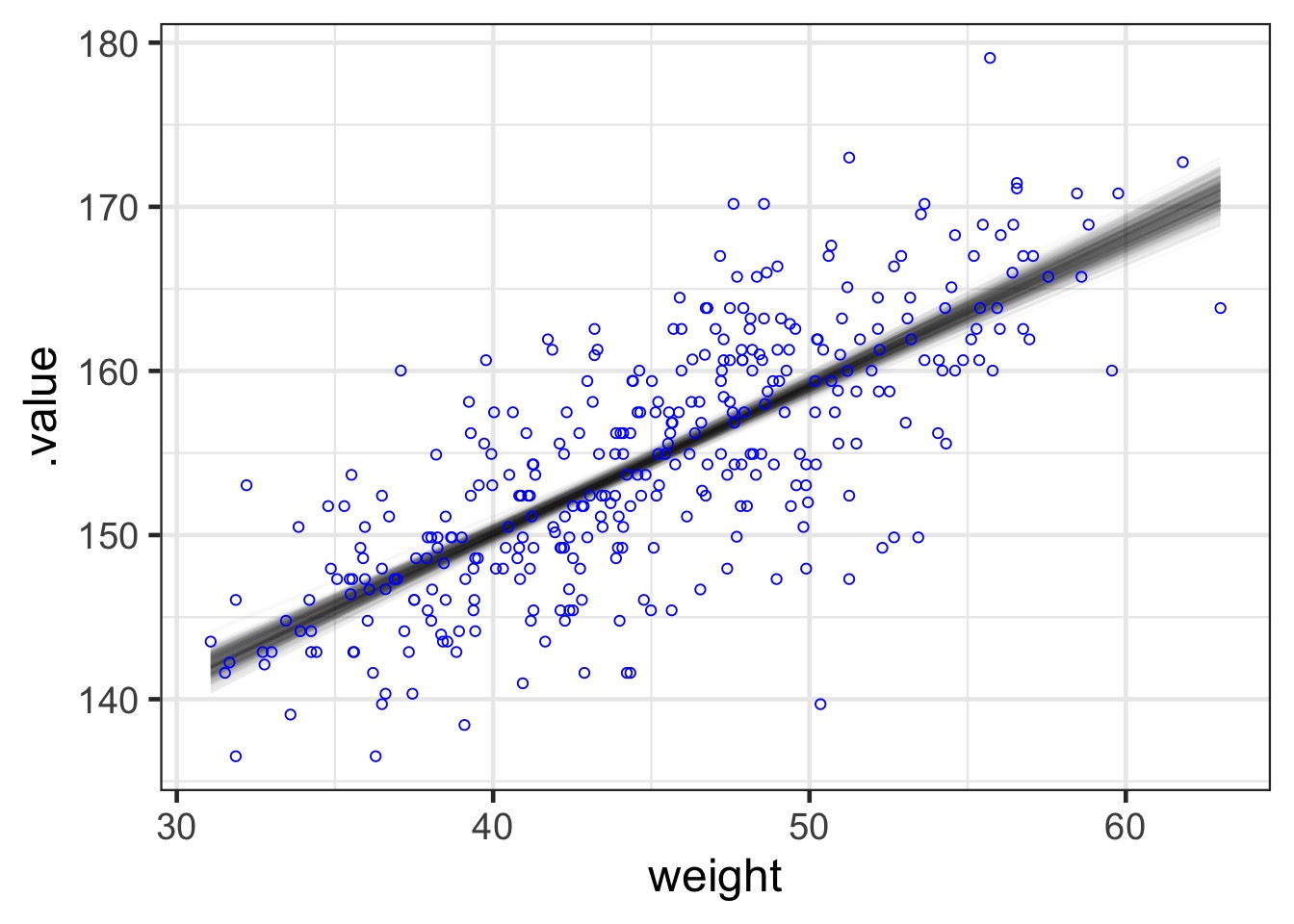
Or, Use ggdist

library(ggdist)
ggplot() +
  
  #simulated fits from the posterior
  stat_lineribbon(data=weight_samps , 
              mapping=aes(x = weight, 
                          y = .value)) +
  
  #the data
  geom_point(data=Howell1_Adult, 
             mapping=aes(x=weight, y=height), pch=1, color = "blue") 

Or, Use ggdist

What about prediction intervals?

#1) Get the posterior prediction interval
pred_samps <- predicted_draws(weight_fit, newdata = Howell1_Adult)


#2) Put it all back together and plot
ggplot() +
  
  #simulated fits from the posterior
  stat_lineribbon(data=pred_samps , 
              mapping=aes(x = weight, 
                          y = .prediction)) +
  
  #the data
  geom_point(data=Howell1_Adult, 
             mapping=aes(x=weight, y=height), pch=1, color = "blue") 

Prediction Interval

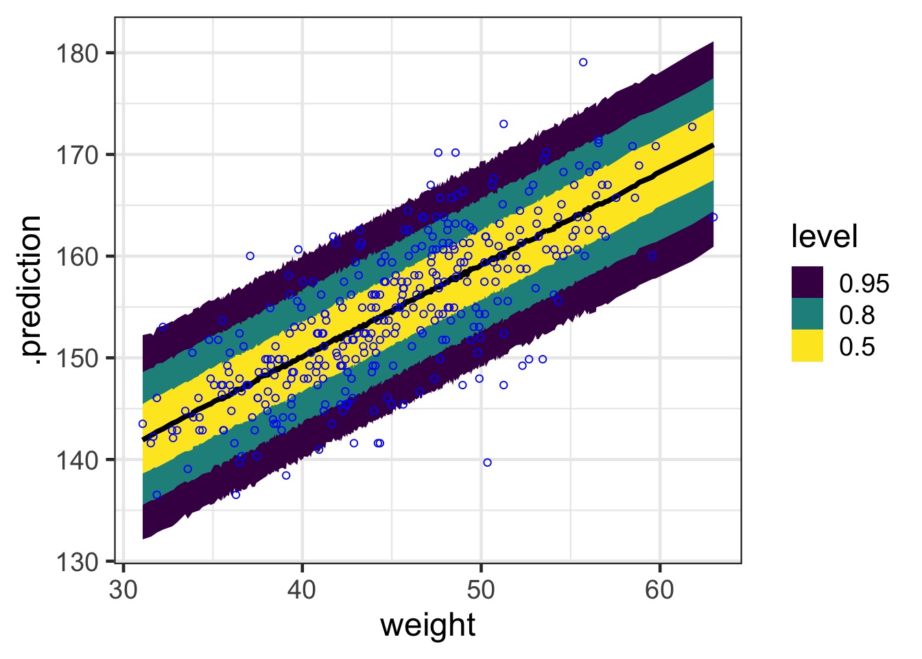
Prediction Interval Lines

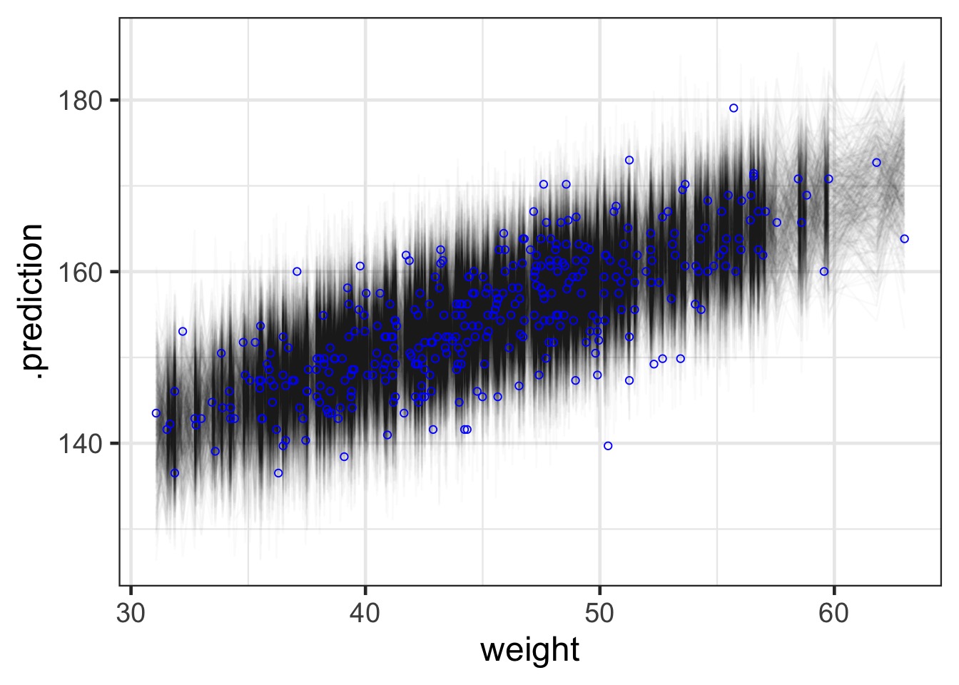
Prediction Interval Points

Polynomial Regression and Standardization

The Actual Data

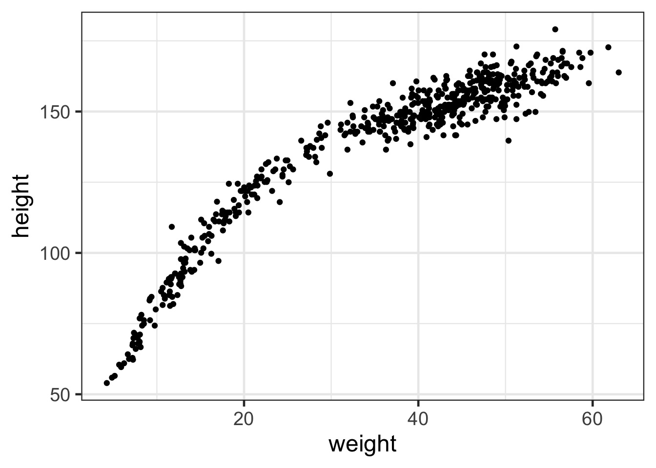
This is not linear!

Before fitting this, Standardize!

• Standardizing a predictor aids in fitting

  • Scale issues of different variables

• Standardizing yields comparable coefficients

• You don’t have to

  • But if you encounter problems, it’s a good fallback

Ye Olde Z Transformation

Howell1 <- mutate(Howell1,
                  weight.s = (weight-mean(weight))/sd(weight))

A Nonlinear Model

Likelihood:
\(h_i \sim Normal( \mu_i, \sigma)\)

Data Generating Process
\(\mu_i = \alpha + \beta_1 x_i + \beta_2 x_i^2 + \beta_3 x_i^3\)

Prior:
\(\alpha \sim \mathcal{N}(150, 20)\)
\(\beta_j \sim \mathcal{N}(0, 10)\)
\(\sigma \sim \mathcal{U}(0,50)\)

Our Model in Code

full_height_mod <- alist(
  #likelihood
  height ~ dnorm(mu, sigma),
  
  #Data generating process
  mu <- alpha + 
    beta1 * weight.s + 
    beta2 * weight.s^2 +
    beta3 * weight.s^3,
  
  #priors
  alpha ~ dnorm(150, 100),
  beta1 ~ dnorm(0, 10),
  beta2 ~ dnorm(0, 10),
  beta3 ~ dnorm(0, 10),
  sigma ~ dunif(0,50)
)

We fit!

full_height_fit <- quap(full_height_mod,
                       data = Howell1)

Before We Go Further, We CAN Look at Priors

In rethinking, we can extract prior coefficients

nonlinear_priors <- extract.prior(full_height_fit)|>
  as_tibble() |>
  mutate(draw = 1:n())

head(nonlinear_priors)

# A tibble: 6 × 6
      alpha     beta1     beta2     beta3     sigma  draw
  <dbl[1d]> <dbl[1d]> <dbl[1d]> <dbl[1d]> <dbl[1d]> <int>
1      91.7    10.3       4.30     -0.299     46.0      1
2     269.     21.6      -2.89     15.5       25.8      2
3     153.      0.101    -0.974     5.86      14.2      3
4     168.    -18.6       2.71     -9.56      43.1      4
5     183.      2.56     -2.95    -14.1       14.0      5
6     198.    -12.2      -9.10     -5.33       7.90     6

We Can Just Calculate Curves

prior_pred <- tidyr::crossing(
  nonlinear_priors[1:100,],
  Howell1 ) |>
  mutate(height = alpha + beta1*weight.s + 
           beta2*weight.s^2 + 
           beta3*weight.s^3)

ggplot(data = Howell1, aes(x = weight.s, y = height)) +
  geom_line(data = prior_pred, aes(group = draw), alpha = 0.5)

Were These Good Priors?

But Did Our Model Fit?

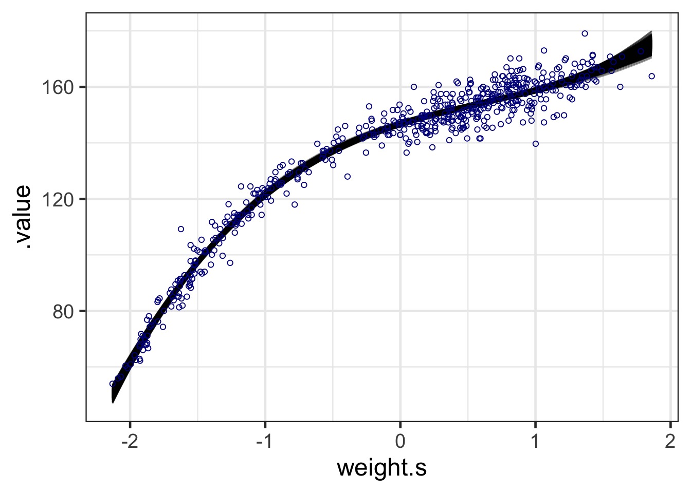
Code

poly_fits <- linpred_draws(full_height_fit, newdata = Howell1,
                           ndraws = 1e3)

ggplot() +
  geom_line(data = poly_fits,
            aes(x = weight.s, y = .value, group = .draw), alpha = 0.4) +
  geom_point(data = Howell1, aes(x = weight.s, y = height),
            pch = 1, color = "darkblue") #+
  #scale_x_continuous(labels = round(-2:2 * sd(Howell1$weight) + mean(Howell1$weight),2))

The Essence of Bayesian Modeling

• Check your data and think about how geocentric you want to be.

• Build a model with reasonable priors

• Test your priors!

  • Don’t be afraid to admit your priors are unrealistic
    
  • If truly worried, test robustness of conclusions to prior choice

• Evaluate the FULL implications of the posterior with samples

  • This includes classic model checks
    
  • But visualize your model fits from samples
    
  • Do you burn down Prague?