Dealing with Autocorrelation

Are Ecological Global Change Analyses Mostly Wrong?

Johnson et al. 2024

Are Ecological Global Change Analyses Mostly Wrong?

Johnson et al. 2024

An Autocorrelated Adventure

Intro to Autocorrelation
Autocorrelation in Space with Gaussian Processes
Autocorrelation due to Phylogeny
Splines and Autocorrelation in Time

Measurements Are Often Distributed in Continuous, Not Discrete, Space

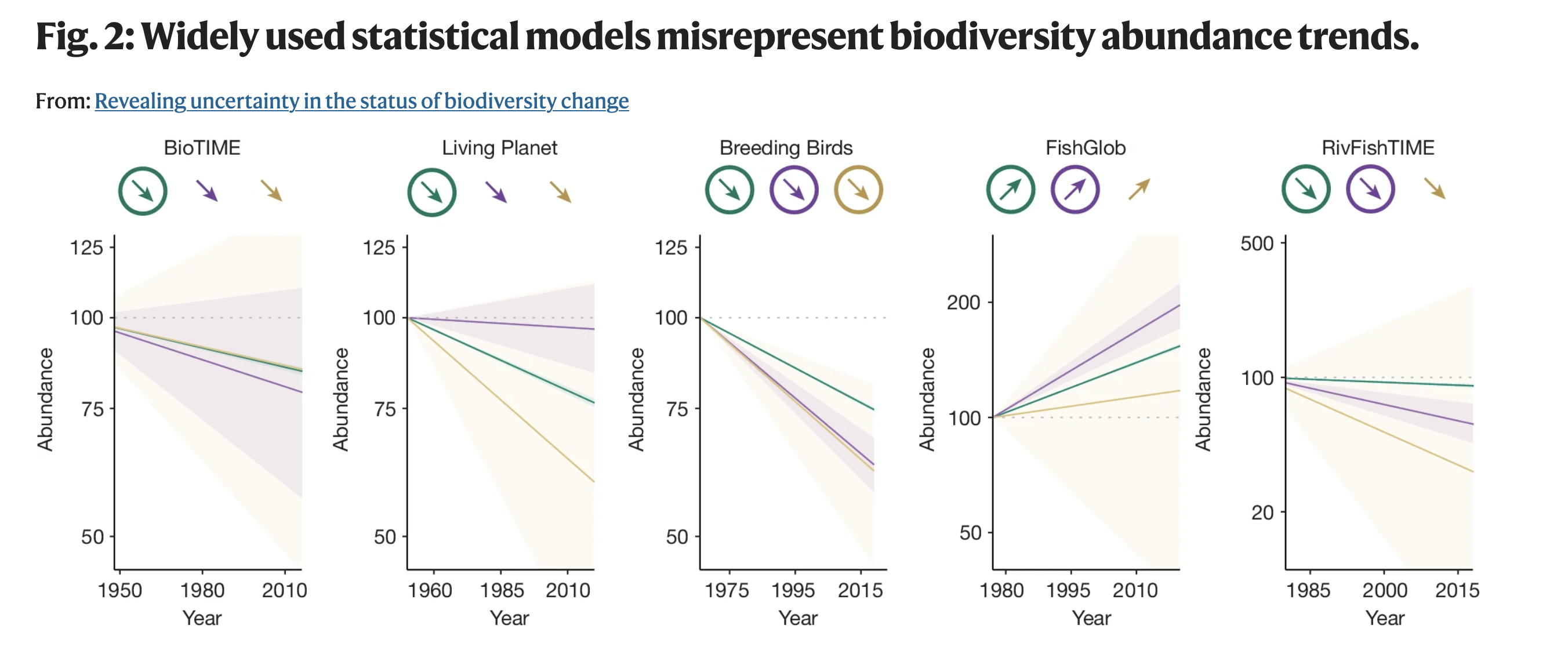
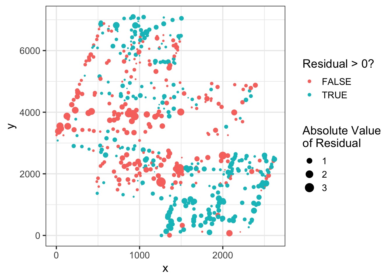
Naive Model

Wetness -> NDVI

boreal <- read.table("./data/06/Boreality.txt", header=T) |>
  mutate(NDVI_s = standardize(NDVI),
         Wet_s = standardize(Wet))


ndvi_nospatial <- alist(
  NDVI_s ~ dnorm(mu, sigma),
  mu <- alpha + beta * Wet_s,
  alpha ~ dnorm(0,1),
  beta ~ dnorm(0,1),
  sigma ~ dexp(2)
)

# fit
ndvi_nospatial_fit <- quap(ndvi_nospatial, boreal)

# residuals
boreal_fit <- linpred_draws(ndvi_nospatial_fit, boreal, ndraws = 1e3) |>
  mutate(.residuals = NDVI_s - .value) |>
  group_by(x, y, point) |>
  summarize(.residuals = mean(.residuals))

Spatial Autocorrelation in Residuals

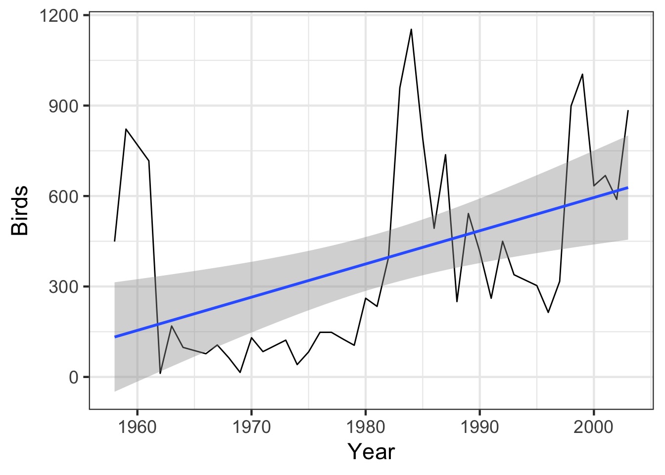
What About Time?

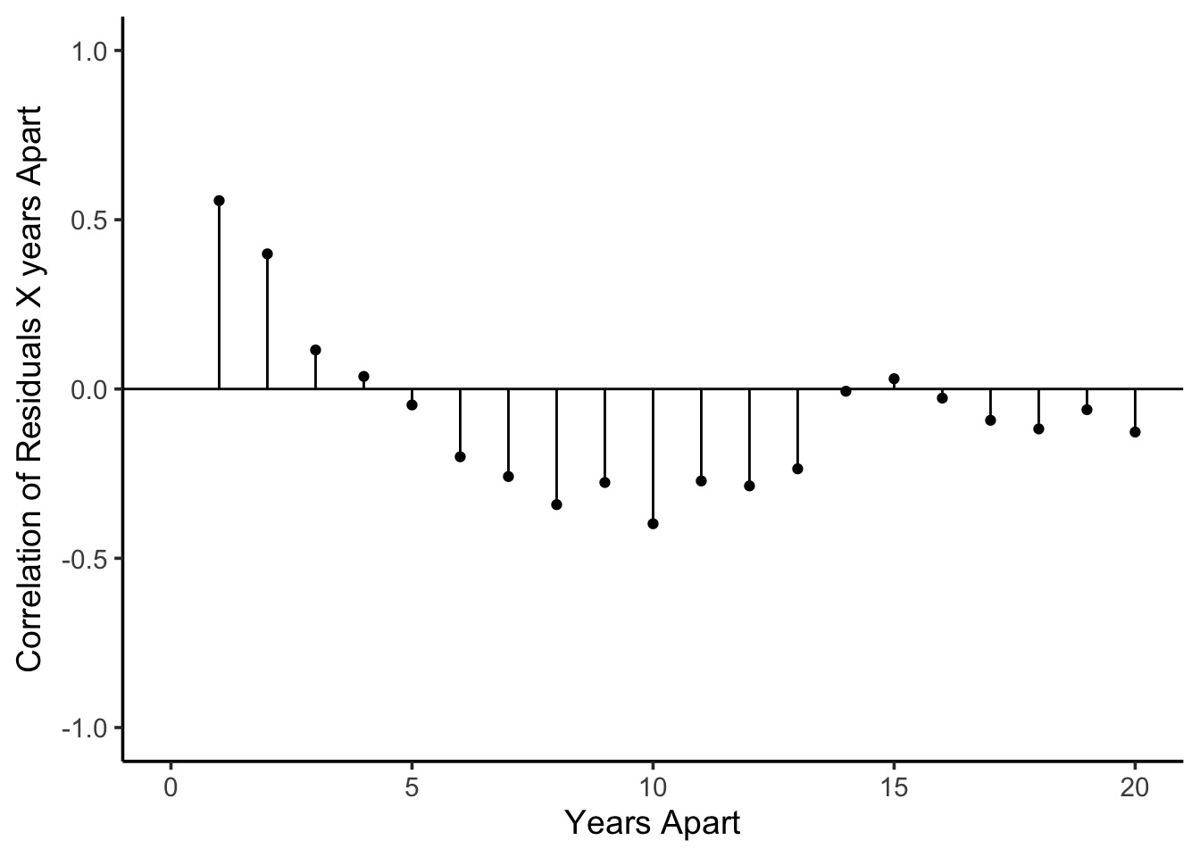
Autocorrelation of Residuals at Different Time Lags

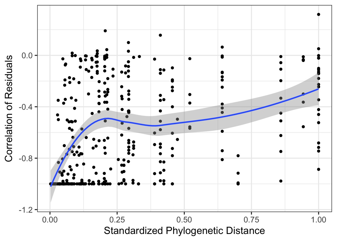
Phylogenetic Autocorrelation

Phylogenetically Correlated Residuals

Considering Correlation: Consider sampling for greeness

Modeling Greeness with a Random Intercept

Likelihood
\(Green_i \sim Normal(\mu_{green}, \sigma_{green})\)

Data Generating Process
\(\mu_{green} = \overline{a} + a_{patch}\)

\(a_{patch} \sim dnorm(0, \sigma_{patch})\)

But “patch” isn’t discrete - it’s continuous, and we know how close they are to each other!

We Think in Terms of a Continuous Correlation Matrices of Residuals

\[cor(\epsilon) = \begin{pmatrix} 1 & \rho_{12} &\rho_{13} \\ \rho_{12} & 1& \rho_{23}\\ \rho_{13} & \rho_{23} & 1 \end{pmatrix}\]

Maybe \(\rho_{12} = \rho_{23} = ...\), maybe there is a function?

For a MVN, We Use the Covariance Matrix

\[K_{ij} = \begin{pmatrix} \sigma_1^2 & \sigma_1\sigma_2 &\sigma_1\sigma_3 \\ \sigma_1\sigma_2 & \sigma_2^2& \sigma_2\sigma_3\\ \sigma_1\sigma_3 & \sigma_2\sigma_3 & \sigma_3^2 \end{pmatrix}\]

But: what is the function that defines \(\sigma_i\sigma_j\) based on the distance between i and j?

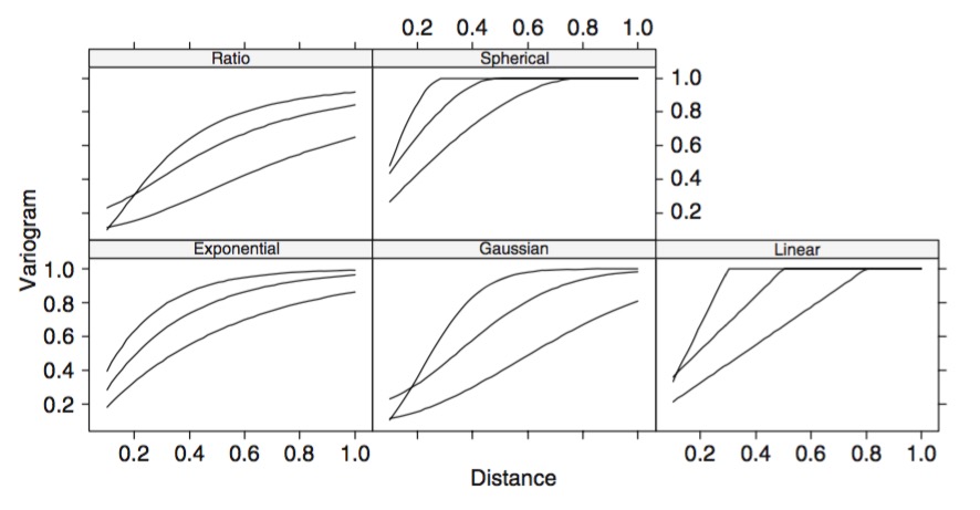
Different Shapes of Autocorrelation

Introducing Gaussian Processes

A GP is a random process creating a multivariate normal distribution between points where the covariance between points is related to their distance.

\[a_{patch} \sim MVNorm(0, K)\]

\[K_{ij} = F(D_{ij})\] where \(D_{ij} = x_i - x_j\)

The Squared Exponential/Gaussian Function(kernel)

\[K_{ij} = \eta^2 exp \left( -\frac{D_{ij}^2}{2 \mathcal{l}^2} \right)\]

where \(\eta^2\) provides the scale of the function and \(\mathcal{l}\) the timescale of the process

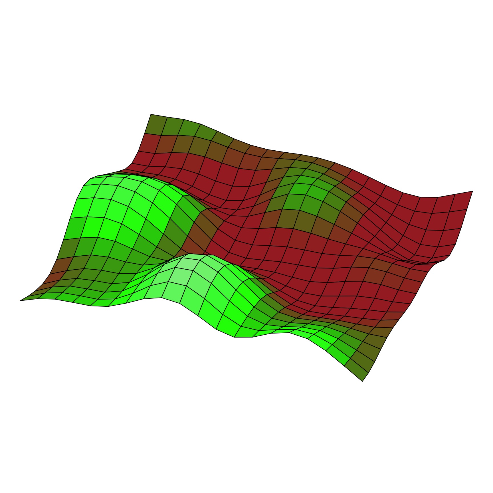
The Squared Exponential Covariance Function (kernel)

A surface from a Squared Exponential GP

Squared Exponential v. Linear Dropoff

Other Covariance Functions

Periodic: \(K_{P}(i,j) = \exp\left(-\frac{ 2\sin^2\left(\frac{D_{ij}}{2} \right)}{\mathcal{l}^2} \right)\)
Ornstein–Uhlenbeck: \(K_{OI}(i,j) = \eta^2 exp \left( -\frac{|D_{ij}|}{\mathcal{l}} \right)\)
Quadratic \(K_{RQ}(i,j)=(1+|d|^{2})^{-\alpha },\quad \alpha \geq 0\)
Note, all of the above can be folded into 1D or 3D, etc autocorrelation
AR1, AR2, etc., are just modifications of the above

The Squared Exponential Function in rethinking (with cov_GPL2)

\[K_{ij} = \eta^2 exp \left( -\frac{D_{ij}^2}{2 \mathcal{l}^2} \right)\]
Rethinking:
\[K_{ij} = \eta^2 exp \left( -\rho^2 D_{ij}^2 \right) + \delta_{ij}\sigma^2\]

\(\rho^2 = \frac{1}{2 \mathcal{l}^2}\)

\(\delta_{ij}\) introduces extra covariance due to replicate measurements

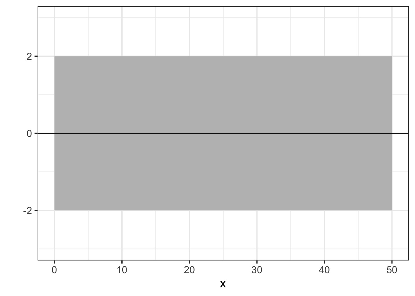
Operationalizing a GP

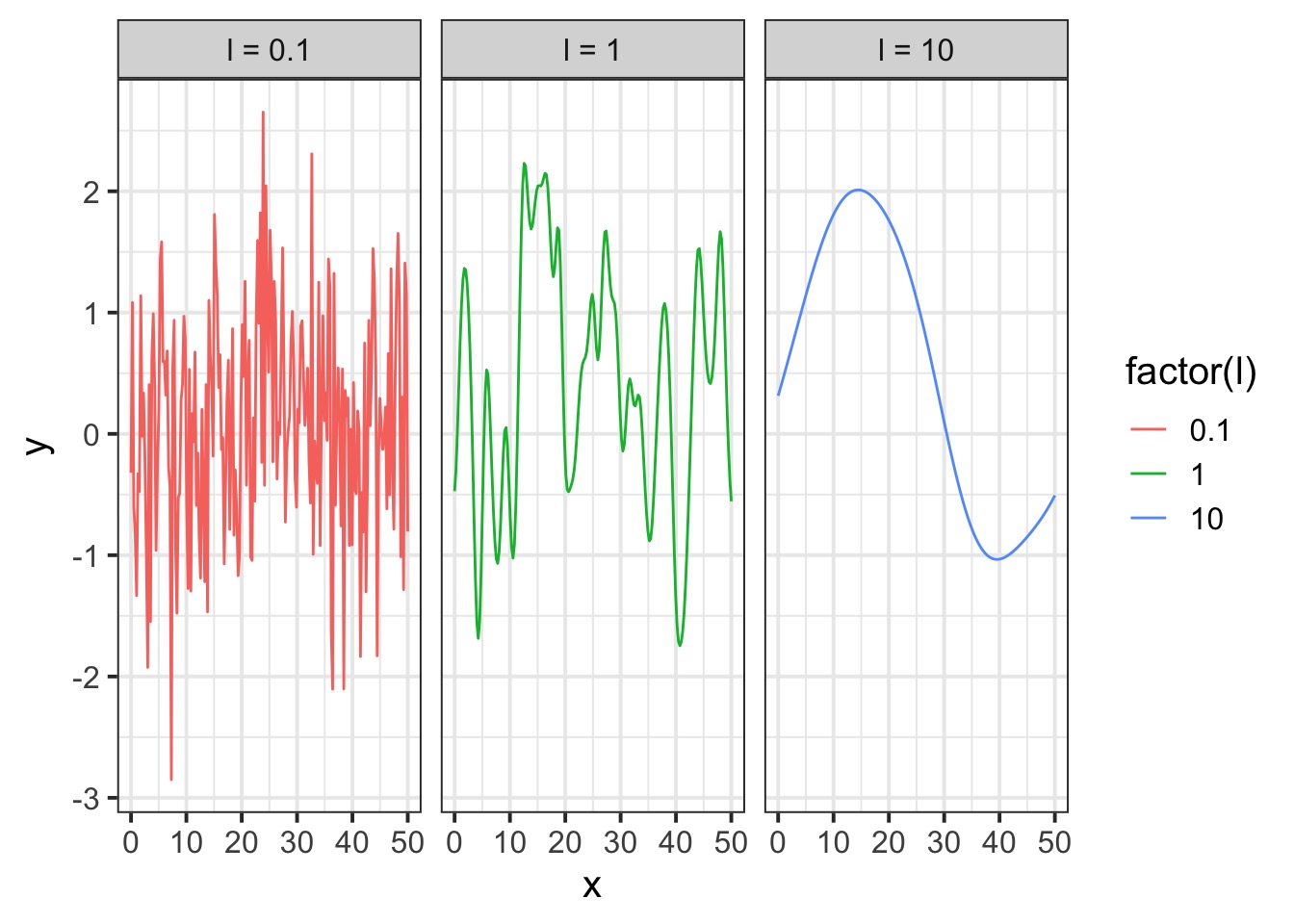
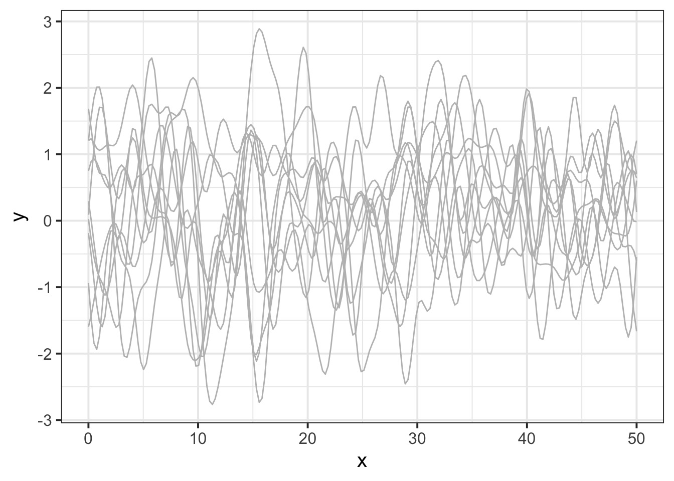
Let’s assume a Squared Exponential GP with an \(\eta^2\) and \(\mathcal{l}\) of 1. Many possible curves:

Operationalizing a GP

And actually, on average

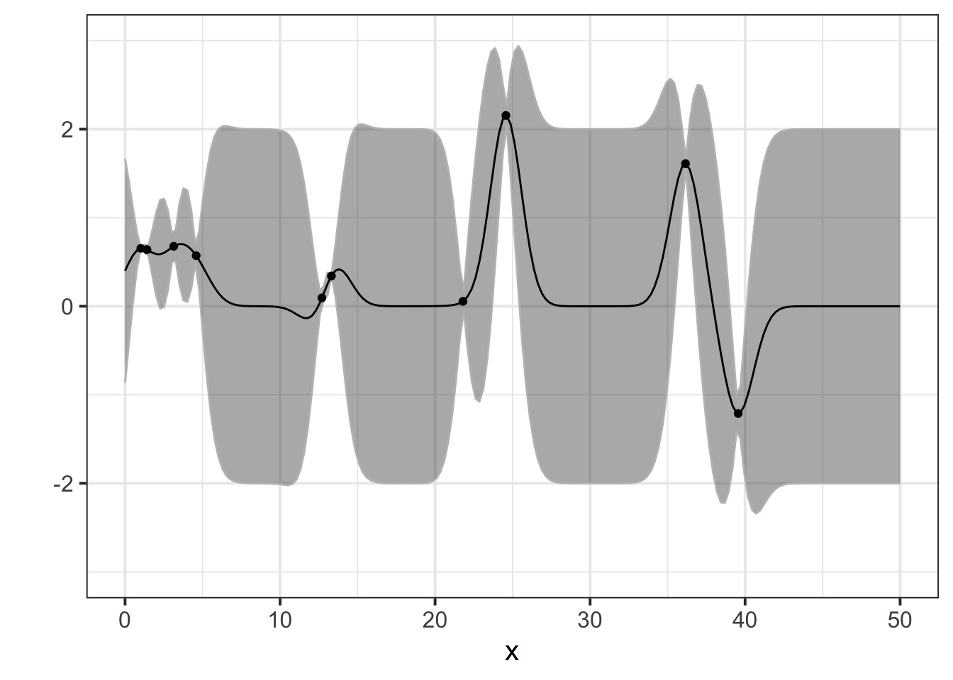
But once we add some data…

Pinching in around observations!

Warnings!

Not mechanistic!
But can incorporate many sources of variability
- e.g., recent analysis showing multiple GP underlying Zika for forecasting
Can mix mechanism and GP

An Autocorrelated Adventure

Intro to Autocorrelation
Autocorrelation in Space with Gaussian Processes
Autocorrelation due to Phylogeny
Splines and Autocorrelation in Time

Oceanic Tool Use

     culture population contact total_tools mean_TU   lat   lon  lon2   logpop
1   Malekula       1100     low          13     3.2 -16.3 167.5 -12.5 7.003065
2    Tikopia       1500     low          22     4.7 -12.3 168.8 -11.2 7.313220
3 Santa Cruz       3600     low          24     4.0 -10.7 166.0 -14.0 8.188689
4        Yap       4791    high          43     5.0   9.5 138.1 -41.9 8.474494
5   Lau Fiji       7400    high          33     5.0 -17.7 178.1  -1.9 8.909235
6  Trobriand       8000    high          19     4.0  -8.7 150.9 -29.1 8.987197

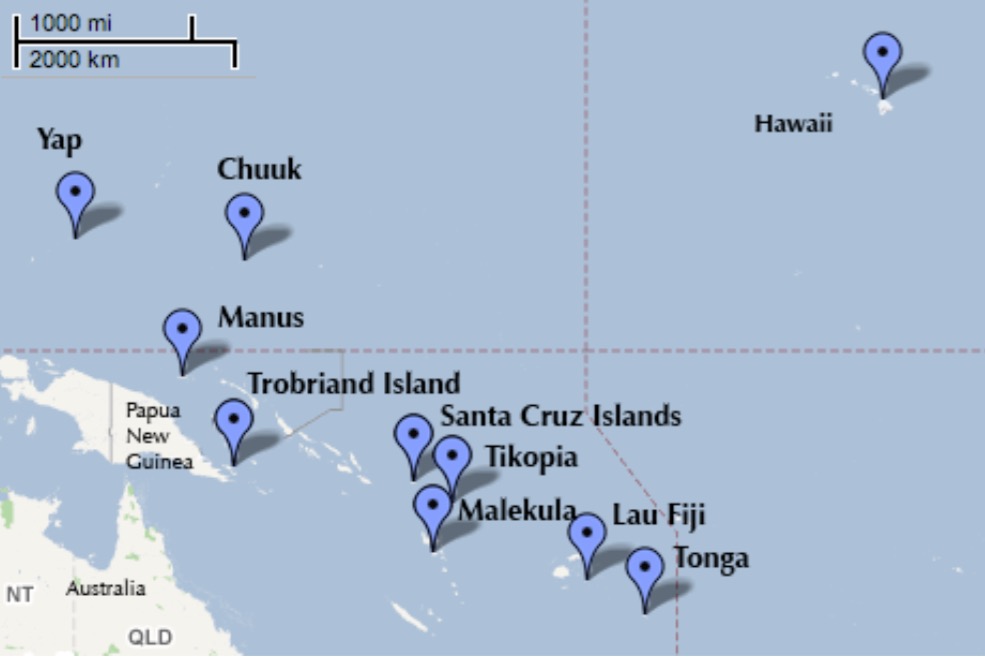
Distances between islands

data(islandsDistMatrix)
islandsDistMatrix

           Malekula Tikopia Santa Cruz   Yap Lau Fiji Trobriand Chuuk Manus
Malekula      0.000   0.475      0.631 4.363    1.234     2.036 3.178 2.794
Tikopia       0.475   0.000      0.315 4.173    1.236     2.007 2.877 2.670
Santa Cruz    0.631   0.315      0.000 3.859    1.550     1.708 2.588 2.356
Yap           4.363   4.173      3.859 0.000    5.391     2.462 1.555 1.616
Lau Fiji      1.234   1.236      1.550 5.391    0.000     3.219 4.027 3.906
Trobriand     2.036   2.007      1.708 2.462    3.219     0.000 1.801 0.850
Chuuk         3.178   2.877      2.588 1.555    4.027     1.801 0.000 1.213
Manus         2.794   2.670      2.356 1.616    3.906     0.850 1.213 0.000
Tonga         1.860   1.965      2.279 6.136    0.763     3.893 4.789 4.622
Hawaii        5.678   5.283      5.401 7.178    4.884     6.653 5.787 6.722
           Tonga Hawaii
Malekula   1.860  5.678
Tikopia    1.965  5.283
Santa Cruz 2.279  5.401
Yap        6.136  7.178
Lau Fiji   0.763  4.884
Trobriand  3.893  6.653
Chuuk      4.789  5.787
Manus      4.622  6.722
Tonga      0.000  5.037
Hawaii     5.037  0.000

What if I needed to make a distance matrix?

dist(cbind(Kline2$lat, Kline2$lon))

            1          2          3          4          5          6          7
2    4.205948                                                                  
3    5.797413   3.224903                                                       
4   39.115214  37.652756  34.444884                                            
5   10.692053  10.754069  13.978913  48.371893                                 
6   18.257053  18.258423  15.231874  22.250393  28.650305                      
7   28.539446  26.152055  23.129418  13.662357  36.500137  16.115210           
8   25.019992  24.158849  20.946837  14.560220  34.882660   7.717513  10.599057
9  342.735029 344.115112 341.361524 314.800540 353.317336 326.339486 328.049082
10 325.121593 325.994172 323.052503 293.884076 335.811629 307.831464 307.454208
            8          9
2                       
3                       
4                       
5                       
6                       
7                       
8                       
9  322.665802           
10 303.298945  45.534273

Well, convert lat/lon to UTM first, and to matrix after dist

Our GP Model

Likelihood
\(Tools_i \sim Poisson(\lambda_i)\)

Data Generating Process \(log(\lambda_i) = \alpha + \gamma_{society} + \beta log(Population_i)\)

Gaussian Process \(\gamma_{society} \sim MVNormal((0, ....,0), K)\)
\(K_{ij} = \eta^2 exp \left( -\rho^2 D_{ij}^2 \right) + \delta_{ij}(0.01)\)

Priors
\(\alpha \sim Normal(0,10)\)
\(\beta \sim Normal(0,1)\)
\(\eta^2 \sim Exponential(2)\)
\(\rho^2 \sim Exponential(0.5)\)

Our model

Kline2$society <- 1:nrow(Kline2)

k2mod <-   alist(
  # likelihood
  total_tools ~ dpois(lambda),
  
  # Data Generating Process
  log(lambda) <- a + k[society] + bp*logpop,

  # Gaussian Process
  vector[10]:k ~ multi_normal( 0 , SIGMA ),
  matrix[10,10]:SIGMA <- cov_GPL2( Dmat , etasq , rhosq , 0.01 ),
  
  # Priors
  a ~ dnorm(0,10),
  bp ~ dnorm(0,1),
  etasq ~ dexp(2),
  rhosq ~ dexp(0.5)
  )

GPL2

g[society] ~ cov_GPL2( Dmat , etasq , rhosq , 0.01)

Note that we supply a distance matrix
cov_GPL2 explicitly creates the MV Normal density, but only requires parameters

Fitting - a list shall lead them

We have data of various classes (e.g. matrix, vectors)
Hence, we use a list
This can be generalized to many cases, e.g. true multilevel models

k2fit <- ulam(k2mod,
 data = list(
    total_tools = Kline2$total_tools,
    logpop = Kline2$logpop,
    society = Kline2$society,
    Dmat = islandsDistMatrix),
 chains=3)

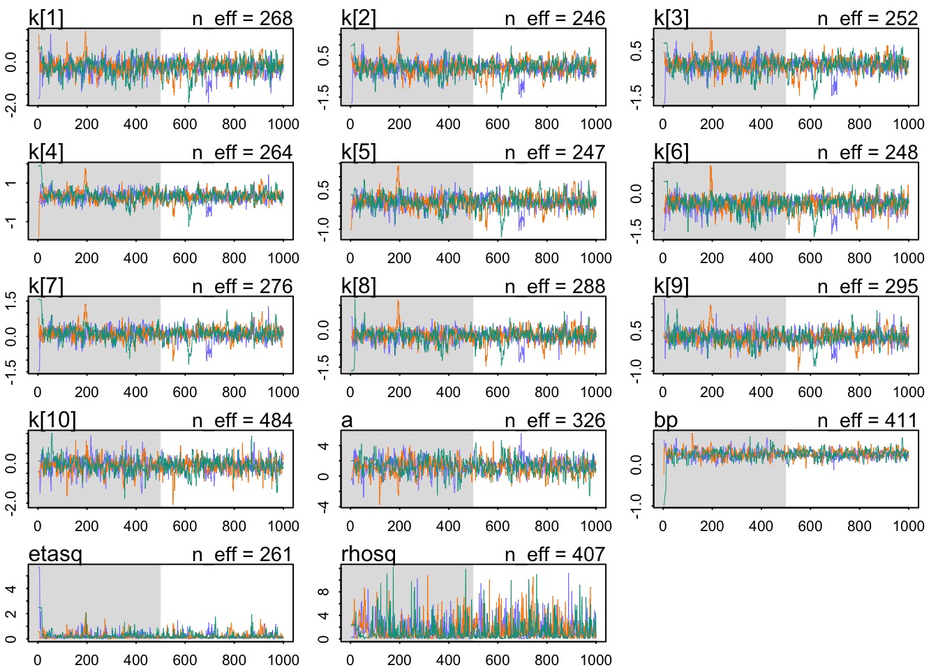
Did it converge?

Did it fit?

What does it all mean?

           mean         sd        5.5%     94.5%     rhat ess_bulk
a     1.2683090 0.96101153 -0.18077277 2.8894966 1.014524 325.8624
bp    0.2486083 0.09600888  0.09306479 0.3967548 1.011408 410.5729
etasq 0.2039891 0.22047529  0.02702730 0.6232529 1.014706 261.0889
rhosq 1.3945047 1.65297194  0.07653043 4.7089869 1.012138 406.8024

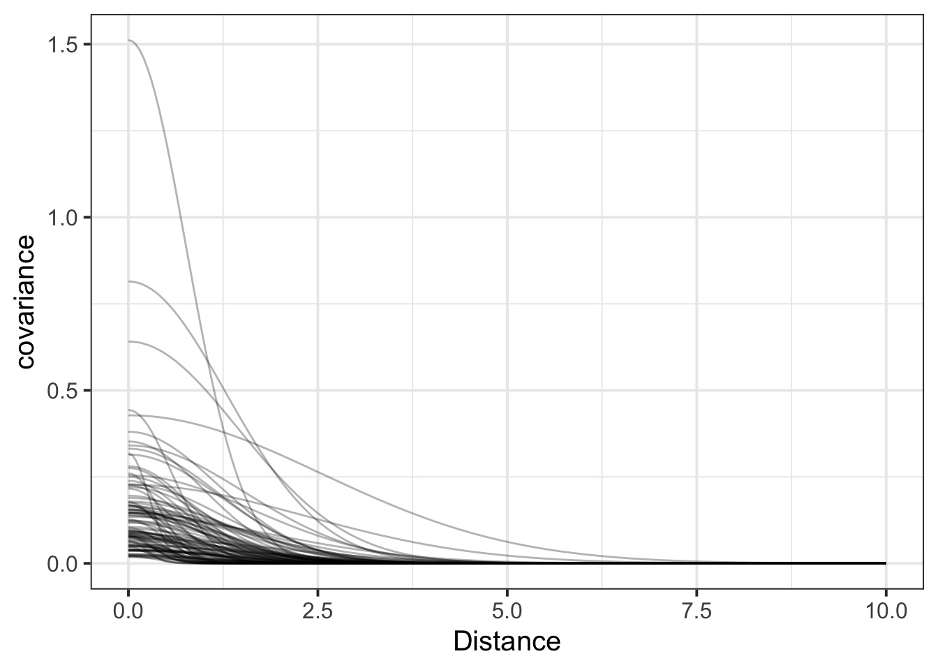
What is our covariance function by distance?

#get samples
k2_samp <- tidy_draws(k2fit) 

#covariance function
cov_fun_rethink <- function(d, etasq, rhosq){
  etasq * exp( -rhosq * d^2)
}

#make curves
decline_df <- crossing(data.frame(x = seq(0,10,length.out=200)), 
                       data.frame(etasq = k2_samp$etasq[1:100],
                                  rhosq = k2_samp$rhosq[1:100])) %>%
 dplyr::mutate(covariance = cov_fun_rethink(x, etasq, rhosq))

Covariance by distance

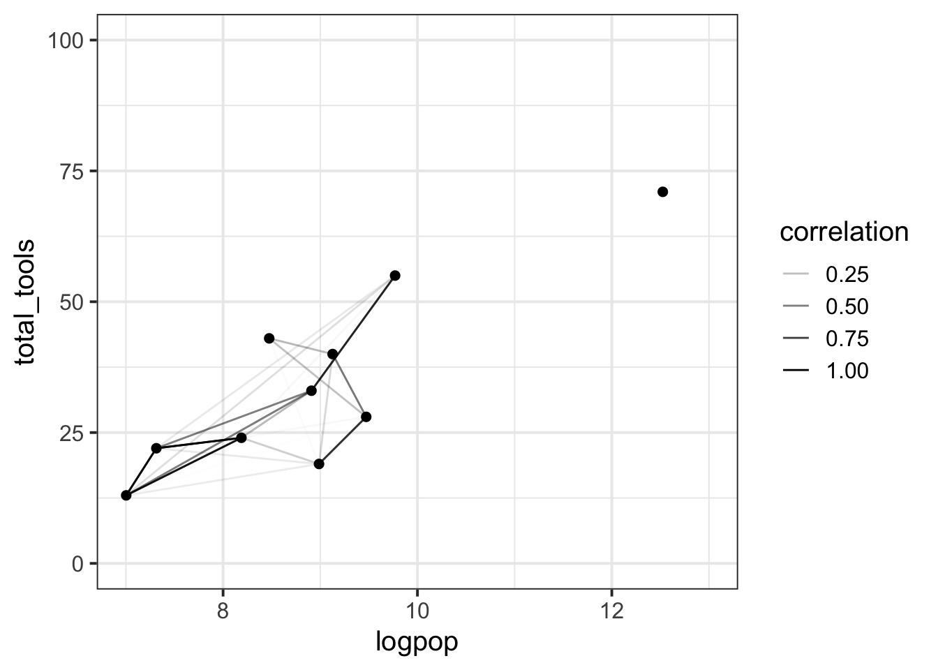
Correlation Matrix

cov_mat <- cov_fun_rethink(islandsDistMatrix,
                           median(k2_samp$etasq),
                           median(k2_samp$rhosq))

cor_mat <- cov2cor(cov_mat)

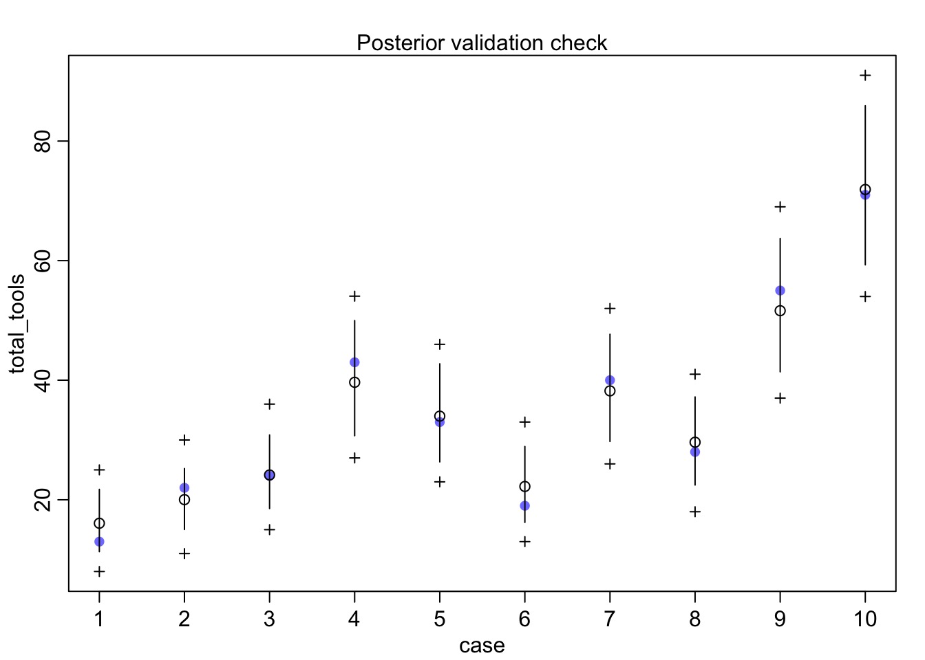
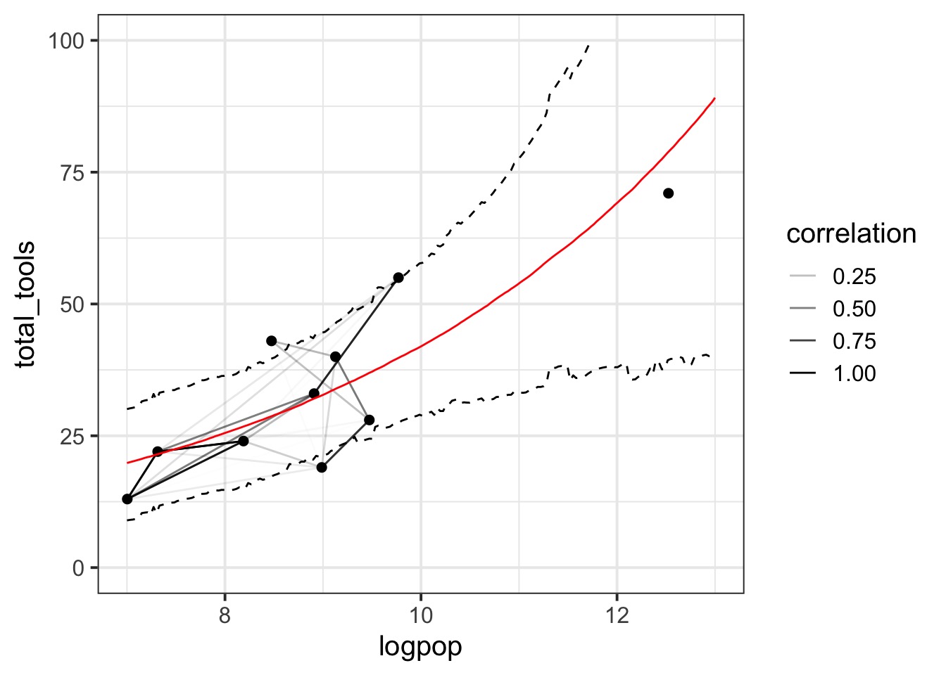
Putting it all together…

An Autocorrelated Adventure

Intro to Autocorrelation
Autocorrelation in Space with Gaussian Processes
Autocorrelation due to Phylogeny
Splines and Autocorrelation in Time

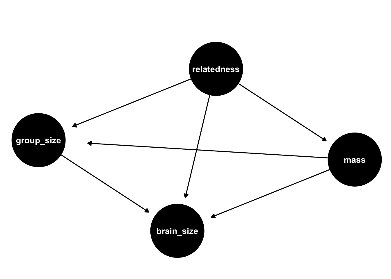
What About Phylogenetic Autocorrelation?

Does Primate Group Size Select for Brain Size?

Possibilities for Incorporating Relatedness

\[group \ size \sim MVN(\mu, \Sigma)\\ \mu_i = \alpha + \beta_G G_i + \beta_M M_i\]

Nothing: \(\Sigma = \sigma^2 I\)
Linear/Brownian: \(\Sigma_{ij} = \rho_{ij} \sigma^2\)
OU/Linear GP: \(K_{ij} = \eta^2 exp \left( -\rho^2 D_{ij} \right)\)

Data Prep

data(Primates301)

dstan <- Primates301 |>
  mutate(name = as.character(name)) |>
  filter(!is.na(group_size),
         !is.na(body),
         !is.na(brain)
         )

# for matrices
spp_obs <- dstan$name

# A list of data and an Identity Matrix
dat_list <- list(
    N_spp = nrow(dstan),
    M = standardize(log(dstan$body)),
    B = standardize(log(dstan$brain)),
    G = standardize(log(dstan$group_size)),
    Imat = diag(nrow(dstan)) )

No Correlation

no_phylo <- ulam(
    alist(
        #likelihood
        B ~ multi_normal( mu , SIGMA ),
        
        # DGP
        mu <- a + bM*M + bG*G,
        
        # Autocorr
        matrix[N_spp,N_spp]: SIGMA <- Imat * sigma_sq,
        
        #priors
        a ~ normal( 0 , 1 ),
        c(bM,bG) ~ normal( 0 , 0.5 ),
        sigma_sq ~ exponential( 1 )
    ), data=dat_list , chains=4 , cores=4)

Making a Correlation Distance Matrix

library(ape)

#make phylo cov/distance matrices
tree_trimmed <- keep.tip( Primates301_nex, spp_obs )
Rbm <- corBrownian( phy=tree_trimmed )
V <- vcv(Rbm)
Dmat <- cophenetic( tree_trimmed )

# put species in right order
dat_list$V <- V[ spp_obs , spp_obs ]

# convert to correlation matrix
dat_list$R <- dat_list$V / max(V)

The Correlation Matrix

Brownian Correlation

brownian <- ulam(
    alist(
        #likelihood
        B ~ multi_normal( mu , SIGMA ),
        
        # DGP
        mu <- a + bM*M + bG*G,
        
        # Autocorr
        matrix[N_spp,N_spp]: SIGMA <- R * sigma_sq,
        
        #priors
         a ~ normal( 0 , 1 ),
        c(bM,bG) ~ normal( 0 , 0.5 ),
        sigma_sq ~ exponential( 1 )
    ), data=dat_list , chains=4 , cores=4, log_lik = TRUE )

OU/Linear GP Correlation

# add scaled and reordered distance matrix
dat_list$Dmat <- Dmat[ spp_obs , spp_obs ] / max(Dmat)

ou_gp_mod <- ulam(
    alist(
        #likelihood
        B ~ multi_normal( mu , SIGMA ),
        
        # DGP
        mu <- a + bM*M + bG*G,
        
        # Autocorr
        matrix[N_spp,N_spp]: SIGMA <- cov_GPL1( Dmat , etasq , rhosq , 0.01 ),        
        #priors
        a ~ normal(0,1),
        c(bM,bG) ~ normal(0,0.5),
        etasq ~ half_normal(1,0.25),
        rhosq ~ half_normal(3,0.25)
        
    ), data=dat_list , chains=4 , cores=4, log_lik = TRUE)

Which Model Fits Best?

#compare(no_phylo, brownian, ou_gp_mod, func = PSIS)

NOTE: Does not currently work due to working with matrices. Standby!

Comparing G

                   mean         sd         5.5%      94.5%     rhat  ess_bulk
no_phylo bG  0.12256875 0.02265879  0.085101822 0.15983441 1.000883 1195.5750
brownian bG  0.02405600 0.02026626 -0.008841488 0.05663509 1.035008  110.6589
ou_gp_mod bG 0.04975294 0.02311785  0.012833085 0.08657639 1.001296 2345.3181

An Autocorrelated Adventure

Intro to Autocorrelation
Autocorrelation in Space with Gaussian Processes
Autocorrelation due to Phylogeny
Splines and Autocorrelation in Time

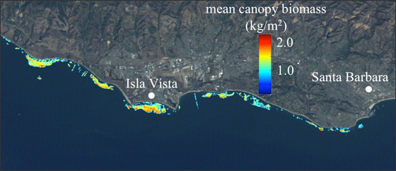
Kelp from spaaaace!!!

Cavanaugh et al. 2011, Bell et al. 2015

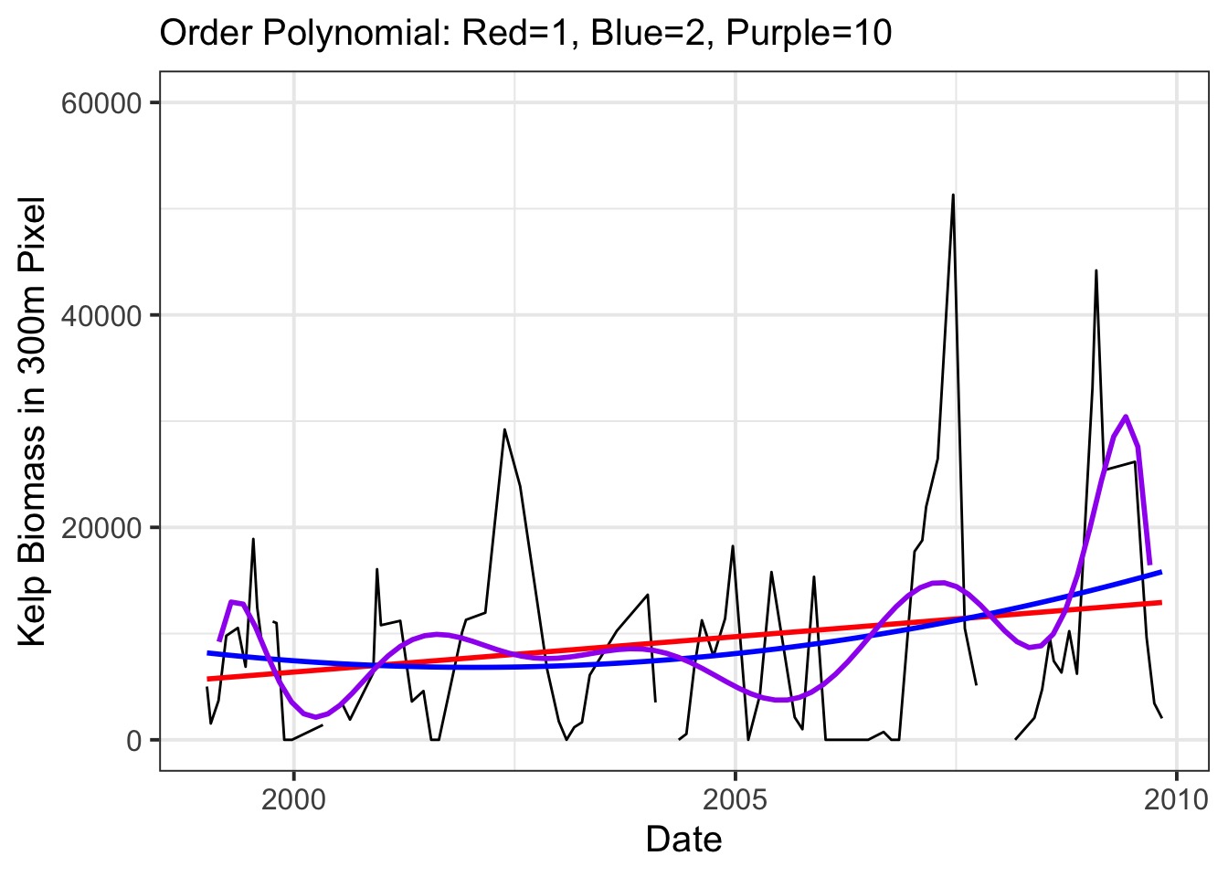
The Mohawk Transect 3 300m Timeseries

Polynomials Only Go So Far

We Can Use Gaussian Processes…

A Gaussian Process is a General Case of a Spline in a Generalized Additive Model

A Spline with many knots converges to a Gaussian Process

How do we Make a Spline: Start

We start with a synthetic variable evenly along the X-axis spread using “knots”

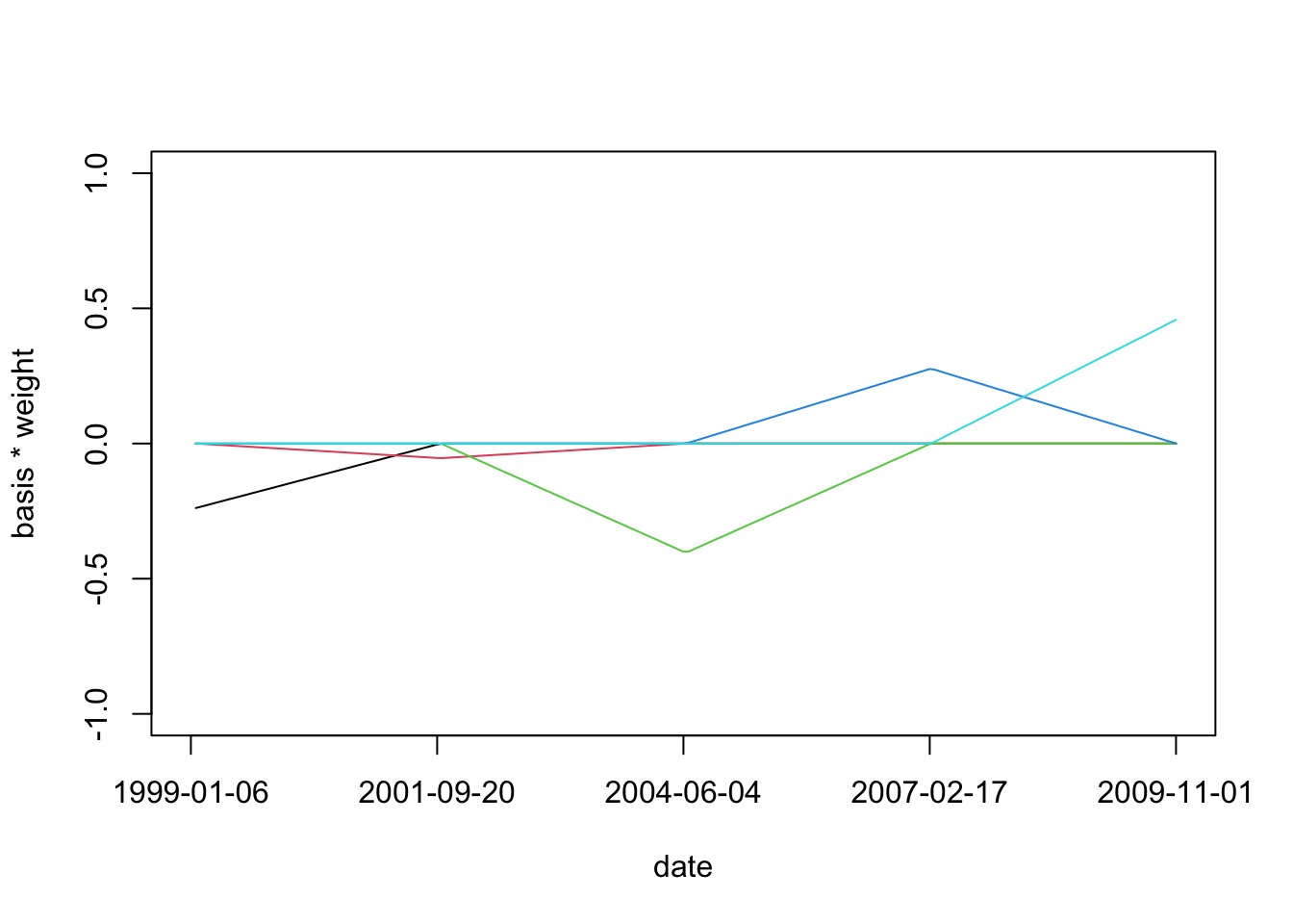
How do we Make a Spline: Weighting

How do we Make a Spline: Sum Weighted Basis Set

Predictions from Spline

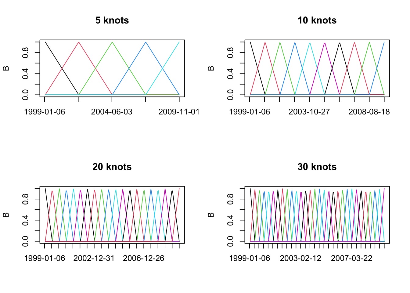
B-Splines with Different Knots

B-Splines of Different Degrees to Control “Wiggliness”

Splines Basis Sets of Different Types

And More…

The GAM Formulation as a Model

Likelihood: \[y_i\sim \mathcal{N}(\mu_i, \sigma^{2})\]

Data Generating Process:
\[g(\mu_i) = f(x_i)\]

\[ f(x_i) = \sum_{j=1}^{d}\gamma_jB_j(x_i)\]

\(B_j(x)\) is your basis function with \(d\) elements.
\(\gamma_j\) is a weight for each element of the basis set.
You can have other linear predictors

The Cental Idea Behind GAMs

Basis Functions: You’ve seen them before

\[f(X) = \sum_{j=1}^{d}\gamma_jB_j(x)\]

Linear Regression as a Basis Function:
\[d = 1\]

\[B_j(x) = x\]

So…. \[f(x) = \gamma_j x\]

Basis Functions: You’ve seen them before

\[f(X) = \sum_{j=1}^{d}\gamma_jB_j(x)\]

Polynomial Regression as a Basis Function:
\[f(x) = \gamma_0 + \gamma_1\cdot x^1 \ldots +\gamma_d\cdot x^d\]

Basis Functions in GAMs

You can think of every \(B_j(x)\) as a transformation of x
In GAMs, we base j off of K knots
A knot is a place where we split our data into pieces
- We optimize knot choice, but let’s just split evenly for a demo
For each segment of the data, we fit a seprate function, then add them together

A Model for the Z-Transformed Kelp Time Series

Likelihood: \[Kelp\:Std_i \sim \mathcal{N}(\mu_i, \sigma)\]

We Z-Transform for ease of fit and to not worry about 0 problem

Data Generating Process: \[\mu_i = \alpha + \sum_{d=1}^D w_d B_{d,i}\]

Here, remember, B is a transform of Date

Priors: \[\alpha \sim \mathcal{N}(0, 2) \\ w_d \sim \mathcal{N}(0, 1) \\ \sigma \sim \mathcal{Exp}(1)\]

Building the Basis Set with 30 knots

# filter NA as it causes problems with matrix multiplication
d <- ltrmk3 |> filter(!is.na(X300m))
d$k_s <- scale(d$X300m)

# make a knot list based on date with 30 knots
knot_list <- seq(min(d$Date), max(d$Date), length.out=30) 

# build the basis set
B <- bs(d$Date,
    knots=knot_list[-c(1,num_knots)], 
    degree=1, 
    intercept=TRUE )

The Model in Rethinking

kelp_spline_mod <- alist(
  # Likelihood
  K ~ dnorm(mu , sigma),
  
  # DGP
  mu <- a + B %*% w,
  
  # Priors
  a ~ dnorm(0, 4),
  w ~ dnorm(0, 1),
  sigma ~ dexp(1)
)

# Fit with start values to give dimensions
# and a list to contain different data types
kelp_spline_fit <- quap(
  kelp_spline_mod,
  data=list( K=d$k_s , B=B) ,
  start=list( w=rep( 0 , ncol(B) ) ) )

What did it all mean?

kelp_pred <- 
  linpred_draws(kelp_spline_fit, 
                newdata = list( K=d$k_s , B=B , Date = d$Date)) |>
  group_by(Date) |>
  summarize(k_s = mean(.value),
            X300m = k_s * sd(d$X300m) + mean(sd(d$X300m)))

What did it all mean?

Space, Time, And All of That

Fundamentally, we assume things close to each other are more similar than things that are far apart.
If our predictors account for all variation, this might not be necessary.
But, if we wish to account for other correlated drivers or autocorrelation in residuals, we have many options
We can model K, the variance-covariance matrix with a MVN process.
We can use a spline (computationally faster) that will approximate a Gaussian Process.
But don’t forget about possible overparameterization…