Prediction and Bayesian Mixed (aka Hierarchical, aka Multilevel) Models


Oceanic Tool Use
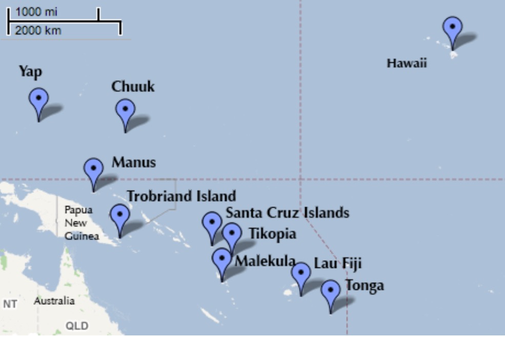
     culture population contact total_tools mean_TU
1   Malekula       1100     low          13     3.2
2    Tikopia       1500     low          22     4.7
3 Santa Cruz       3600     low          24     4.0
4        Yap       4791    high          43     5.0
5   Lau Fiji       7400    high          33     5.0
6  Trobriand       8000    high          19     4.0

Model of Tool Use with Random Variation

Note a_hat’s location to facilitate consructing predictions and efficiency

Kline$society <- 1:nrow(Kline)
Kline$log_pop <- log(Kline$population)

kline_mixed <- alist(
  #Likelihood
  total_tools ~ dpois(lambda),
  
  #DGP
  log(lambda) ~ a_hat + a[society] + bp*log_pop,
  
  a[society] ~ dnorm(0, sigma_society),

  #Priors
  a_hat ~ dnorm(0,10),
  bp ~ dnorm(0,1),
  sigma_society ~ dcauchy(0,2)
)

kline_mixed_fit <- map2stan(kline_mixed, data=Kline,
                            iter=10000, chains=3)

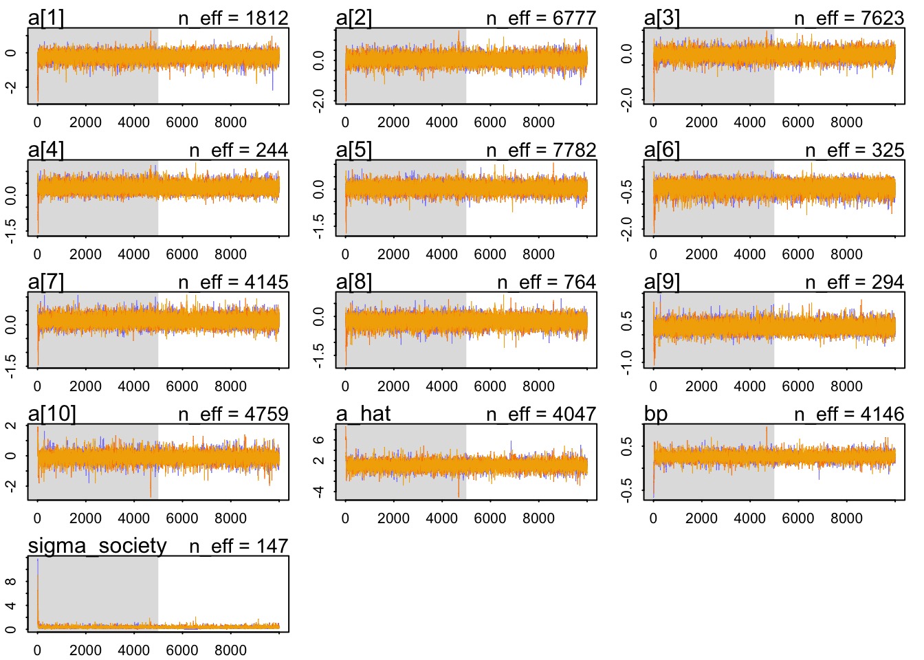
Convergence!

What are we trying to predict with multilevel models?

  1. Prediction based on average “fixed” effect?

  2. Prediction for one bock - new or old!

  3. Prediction marginalized over any possible random effects?
    • Incorporates variance of random effects

Prediction of the Average

  • Use link to get predicted values

  • But, substitute in 0 for the random effects


#nrow = # of sims
a_fixed_mat_zeroes <- matrix(rep(0, 10*1000), nrow=1000, ncol=10)

Compare Fixed Fit Error to Sample Fit Error
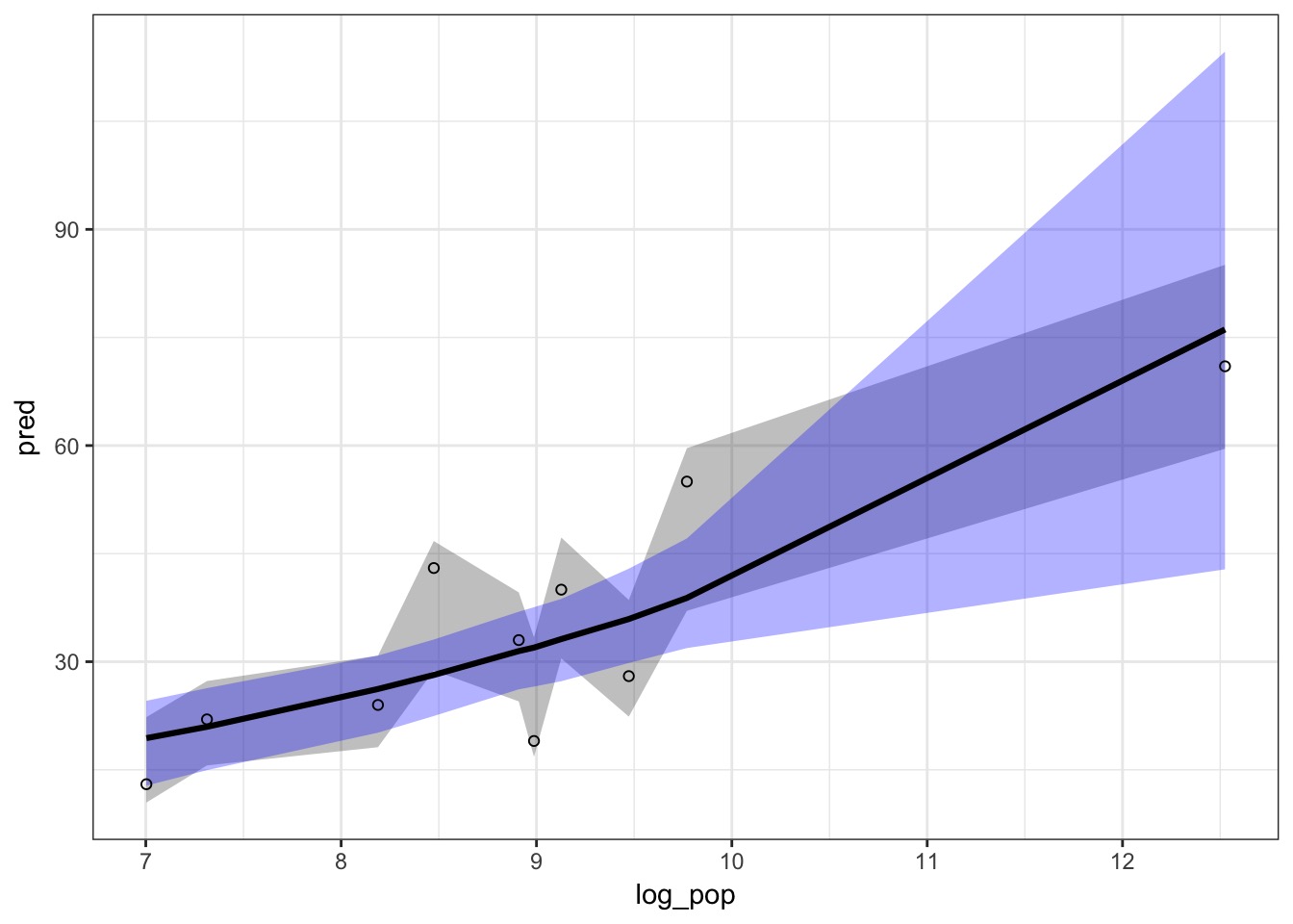
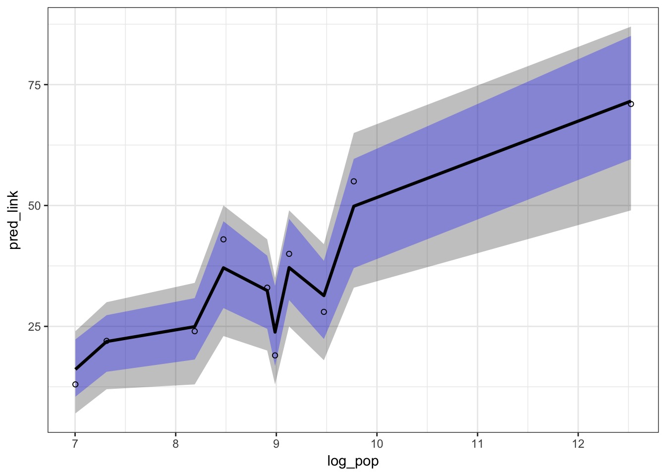
Fit and Prediction Error for Fixed Effects Only
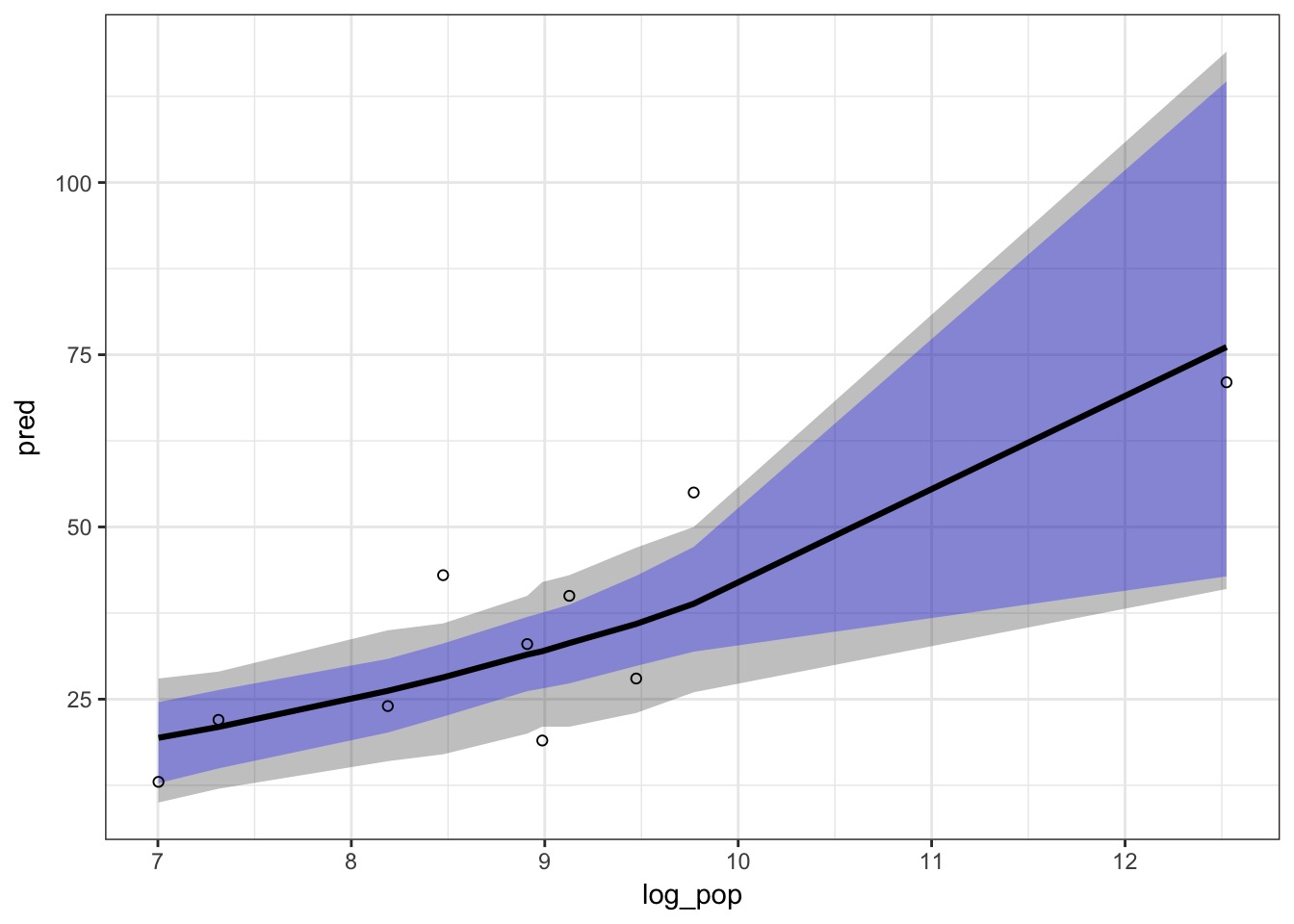
What if we had a new blocks, and wanted their trend?

  • For a single block, a single draw of the random effect will suffice

  • Use the same way as the fixed only model

  • Draw of random effects comes from using the \(\sigma_{society}\) in this case

  • But, parameters values must come from same draws of \(\sigma_{society}\)

Merge New Random Effects

# replace matrices of random effects
kline_samp <-kline_samp[setdiff(names(kline_samp), "a")]

# make into data frame
kline_samp <- as.data.frame(kline_samp)

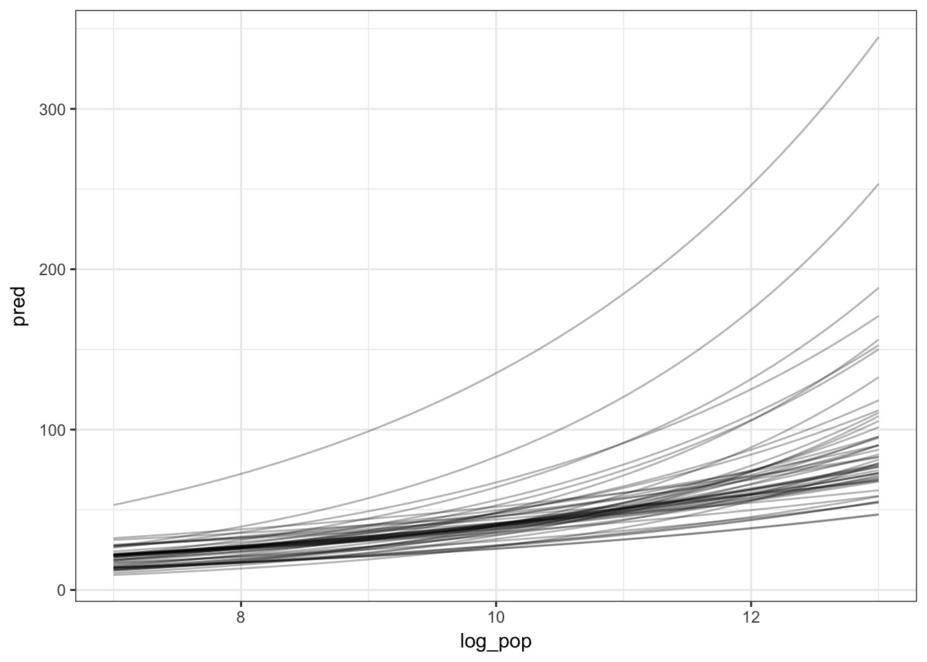
New data frame for plotting

# now make a new data frame
pred_df <- crossing(log_pop = seq(7,13, length.out=100), 
                    kline_samp) %>%
  
    mutate(pred = exp(a_new + a_hat + bp*log_pop))


#plot
ggplot(pred_df, mapping=aes(x=log_pop, y=pred, group=a_new)) +
  geom_line(alpha=0.3)

What if we want to see full distribution of possible new observations

  • a[society] ~ dnorm(0, sigma_society) implies any new society is drawn from that distribution

  • Hence, in addition to fit and prediction uncertainty, we also have new block uncertainty

  • Straightforward to see both fit and prediction error

  • We are marginalizing over random effects

Build that new random effects matrix!

Need as many samples as outputs from sim and link
10 “blocks” * 1000 sims

n_pts <- 10*1000
kline_samp_all <- extract.samples(kline_mixed_fit, n=n_pts)

## New random effects
new_ranefs <- rnorm(n_pts, 0, kline_samp_all$sigma_society)

## New matrix
a_ranef_new <- matrix(new_ranefs, ncol=10, nrow=1000)

Marginalized Counterfactual Predictions
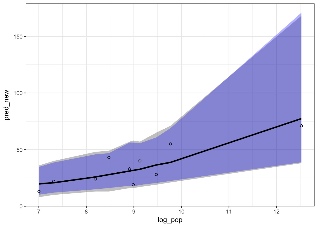
Suggests random effects uncertainty is large relative to prediction uncertainty

Exercise: DINOSAURS!!!!
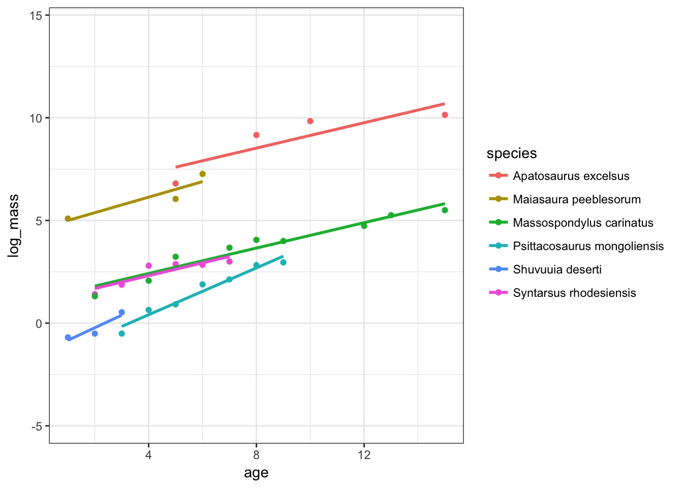
  • Make predictions with fixed effects only and one other