Varying Slopes in Bayesian Mixed (aka Hierarchical, aka Multilevel) Models

Gender Discrimination in Graduate Admissions

Our data: Berkeley

data(UCBadmit)
class(UCBadmit) <- "data.frame"
head(UCBadmit)

  dept applicant.gender admit reject applications
1    A             male   512    313          825
2    A           female    89     19          108
3    B             male   353    207          560
4    B           female    17      8           25
5    C             male   120    205          325
6    C           female   202    391          593

A Poor First Model

#Make a dept and genderindex
UCBadmit$gender <- as.numeric(UCBadmit$applicant.gender)
UCBadmit$dept_id <- as.numeric(UCBadmit$dept)

mod_gender_bad <- alist(
  #likelihood
  admit ~ dbinom(applications, p),
  
  #Data generating process
  logit(p) <- a + b[gender],
  
  #priors
  a ~ dnorm(0,10),
  b[gender] ~ dnorm(0,10)
)

fit_gender_bad <- quap(mod_gender_bad, UCBadmit)

How does it look?

What is the model we want?

Random effect of departent
- Recall a fixed effect of department fit much better
AND the gender effect might vary by department
- In fixed effects, this would be dept*gender
- In mixed models, effect of gender varies by department

What about this?

\(a_{dept} \sim dnorm(\hat{a}, \sigma_{a})\)

\(b_{dept} \sim dnorm(\hat{b}, \sigma_{b})\)

What is missing?

Notice how Slope and Intercept covary

Dealing with Slope-Intercept Covariance

So, if we want… \[logit(p_i) = a_{dept} + b_{dept} gender_i\]

Then, \(a_{dept}\) and \(b_{dept}\) must covary

\[\begin{bmatrix} a_{dept} \\ b_{dept} \end{bmatrix} \sim MVNormal \left (\begin{bmatrix} \widehat{a} \\ \widehat{b} \end{bmatrix}, \textbf{S} \right )\]

Building a Covariance Matrix with Correlations

A covariance matrix is fine, but we often want to know correlation
Often harder to parameterize a covariance matrix conceptually
Fortunately, cov_ab = cor_absd_asd_b

\[S_{ab} = \begin{bmatrix} \sigma_a & 0\\ 0 & \sigma_b \end{bmatrix} \begin{bmatrix} 1& r_{ab}\\ r_{ab} & 1 \end{bmatrix} \begin{bmatrix} \sigma_a & 0\\ 0 & \sigma_b \end{bmatrix}\]

Priors and Correlations

We know about how to make \(\sigma\) priors with dcauchy
What about correlations?
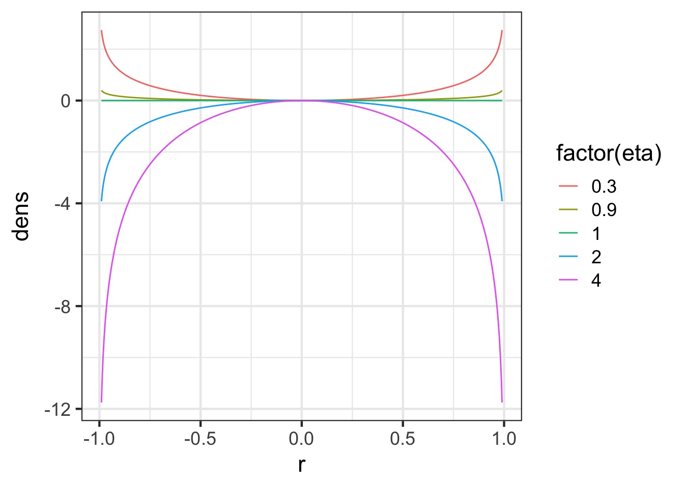
Introducting, the LKJ Correlation Distribution!

-Evaluates probability of correlation matrices

-Parameter \(\eta\) says how peaked it is towards 0

LKJ Correlation Distribution

So, those random effects…

\[\begin{bmatrix} a_{dept} \\ b_{dept} \end{bmatrix} \sim MVNormal \left (\begin{bmatrix} \widehat{a} \\ \widehat{b} \end{bmatrix}, \mathbf{ \sigma } \textbf{R} \mathbf{ \sigma } \right )\]

A Variable Slope Intercept Model

UCBadmit$isMale <- as.numeric(UCBadmit$applicant.gender)-1

mod_gender_dept_mixed <- alist(
  #likelihood
  admit ~ dbinom(applications, p),
  
  #Data generating process
  logit(p) <- a_hat + a[dept_id] + b_hat*isMale + b[dept_id]*isMale,
  
  # RE
  c(a,b)[dept_id] ~ multi_normal(c(0,0), Rho, sigma_dept),
  
  #priors
  a_hat ~ dnorm(0,10),
  b_hat ~ dnorm(0,10),
  
  sigma_dept ~ dexp(2),
  Rho ~ dlkjcorr(2)
)

What is new

Our definition of random effects:
c(a,b)[dept_id] ~ dmvnorm2(c(0,0),
sigma_dept, Rho)

sigma_dept knows there are 2 values:
sigma_dept ~ dexp(2)

Our Correlation Prior:
Rho ~ dlkjcorr(2)

Fitting

fit_gender_dept_mixed <- ulam(mod_gender_dept_mixed, 
                              
                              UCBadmit |>
                                select(isMale, dept_id, 
                                       admit, applications),
                              
                              chains=3)

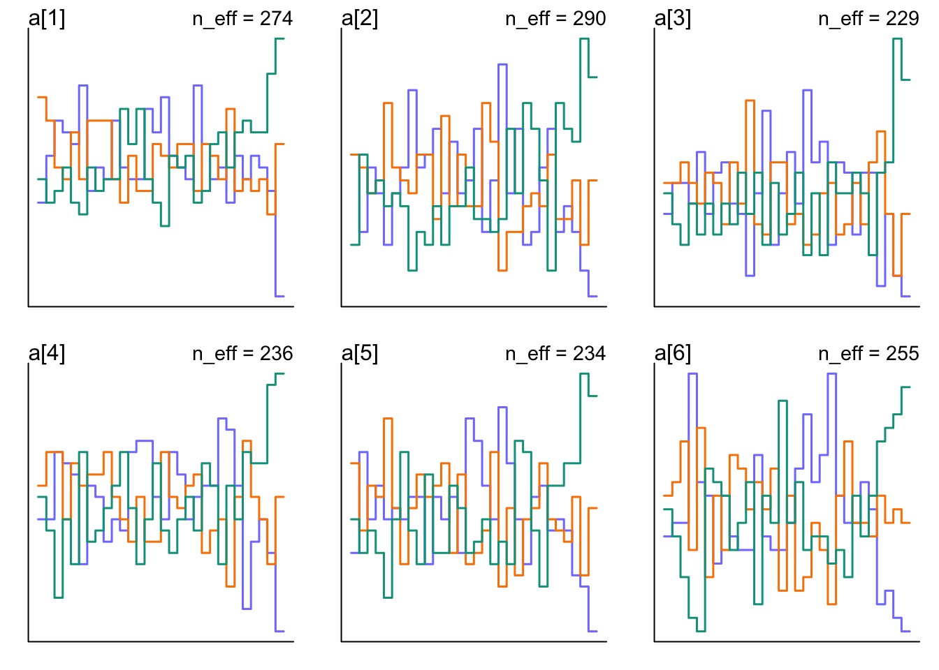
Did it blend?

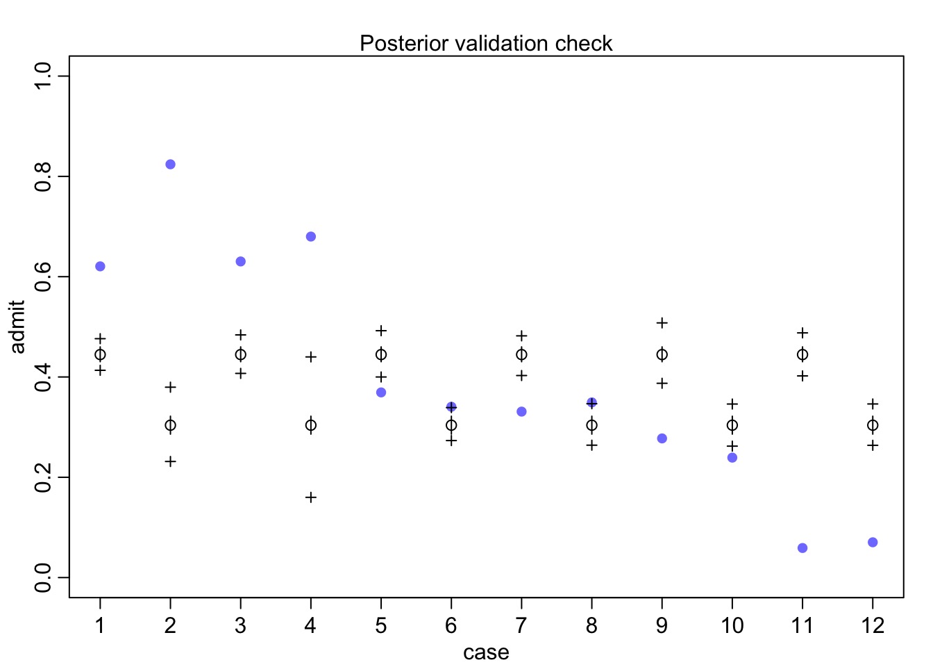
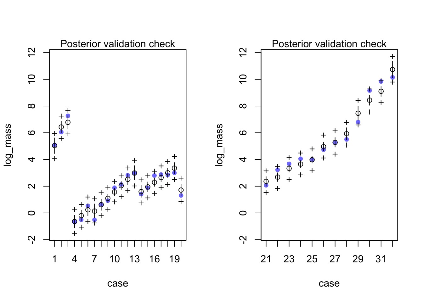
Posterior Check

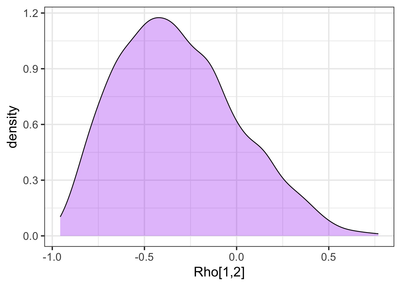
How correlated were slope and intercept?

gender_samp <- tidy_draws(fit_gender_dept_mixed)

ggplot(data = gender_samp, aes(x = `Rho[1,2]`)) +
  geom_density(fill = "purple", alpha = 0.3)

 [1] "lp__"          "b[1]"          "b[2]"          "b[3]"         
 [5] "b[4]"          "b[5]"          "b[6]"          "a[1]"         
 [9] "a[2]"          "a[3]"          "a[4]"          "a[5]"         
[13] "a[6]"          "a_hat"         "b_hat"         "sigma_dept[1]"
[17] "sigma_dept[2]" "Rho[1,1]"      "Rho[2,1]"      "Rho[1,2]"     
[21] "Rho[2,2]"      "treedepth__"   "divergent__"   "energy__"     
[25] "accept_stat__" "stepsize__"    "n_leapfrog__"  ".chain"       
[29] ".iteration"    ".draw"

How correlated were slope and intercept?

How important was incorporating a random slope?

Can look at density of \(\sigma\) for slope and intercept
Can fit variable intercept only model and compare with WAIC
- And no reason you can’t use ensemble predictions if both are valid hypotheses

Density of Sigmas

gender_samp <- gender_samp |>
  rename(sigma_int = `sigma_dept[1]`,
         sigma_slope = `sigma_dept[2]`,
         )

gender_samp |>
  select(sigma_int, sigma_slope) |>
  pivot_longer(cols = everything()) |>
ggplot(aes(x=value, color=name)) +
  geom_density()

Variable Intercept Only Model

mod_gender_dept_varint <- alist(
  #likelihood
  admit ~ dbinom(applications, p),
  
  #Data generating process
  logit(p) <- a_hat + a[dept_id] + b_hat*isMale,
  
  a[dept_id] ~ dnorm(0, sigma_dept),
  
  #priors
  a_hat ~ dnorm(0,10),
  b_hat ~ dnorm(0,10),
  
  sigma_dept ~ dexp(2)
)

fit_gender_dept_varint<- ulam(mod_gender_dept_varint, 
                               data = UCBadmit |>
                                select(isMale, dept_id, 
                                       admit, applications),
                              chains=3)

Not quite as good of a fit…

(I assume we’ve checked the chains…)

WAIC suggests Variable Slope model better…

But big SE - what would you do?

Optimization and Alternate Parameterization

How we build our golem in part of the model itself
We have seen even with centering that we can improve fit/speed
With big multivariate normal densities, Non-centered parameterization can help

Non-Centered Parameterization

Consider
\[ y \sim Normal(\mu, \sigma)\]

This can be re-written as:
\[y = \mu + z \sigma\] \[ z \sim Normal(0,1)\]

Fitting N(0,1) and estimating \(\mu\) and \(z\) is much more efficient

Implications of Non-Centered Parameterization with Mixed Models

NC Paramterization implies that if we pull out sigmas and coefficients, we’re left with mean 0 and a correlation matrix
Correlations of the priors can be further removed with Cholesky decomposition of the correlation matrix
Thus, we can often sample more efficiently
Rethinking does this for you under the hood with dmvnormNC
- Assumes random effects are centered on 0

NC Paramterized Model

mod_gender_dept_nc <- alist(
  #likelihood
  admit ~ dbinom(applications, p),
  
  #Data generating process
  logit(p) <- a_hat + re_dept[dept_id,1] +
    b_hat*isMale + re_dept[dept_id,2]*isMale,
  
  
  # NCP RE
  transpars > matrix[6, 2]:re_dept <- 
    compose_noncentered(sigma_dept, Rho_dept, z_dept),


  #priors
  a_hat ~ dnorm(0,10),
  b_hat ~ dnorm(0,10),
  
  # NCP priors
  matrix[2,6]:z_dept ~ normal( 0 , 1 ),
  vector[2]:sigma_dept ~ dexp(2),
  cholesky_factor_corr[2]:Rho_dept ~ lkj_corr_cholesky( 2 ),
  
  # convert Cholesky to Corr matrix
  gq> matrix[2,2]:Rho <<- Chol_to_Corr(Rho_dept)
)

What is going on in this model matrices

  #Data generating process
  logit(p) <- a_hat + re_dept[dept_id,1] +
    b_hat*isMale + re_dept[dept_id,2]*isMale,

We are using a matrix of random effects.
Can be efficient for large amounts of REs

Our NCP RE Matrix

  # NCP RE
  transpars > matrix[6, 2]:re_dept <- 
    compose_noncentered(sigma_dept, Rho_dept, z_dept),

transpars > says we are creating transformed parameters.
note we define a 6 x 2 matrix of REs - intercepts (col 1) and slopes (col 2).
z_dept is now a z-scored hyperprior for our REs

Our Z-Scored Hyperprior

  # NCP priors
  matrix[2,6]:z_dept ~ normal( 0 , 1 ),

note the matrix is transposed
but, every element is N(0,1)

Our Hyperprior for Departmental Variances

  vector[2]:sigma_dept ~ dexp(2),

we declare a vector of sigmas for intercept and slope
but otherwise as before

Our Correlation Matrix

  cholesky_factor_corr[2]:Rho_dept ~ lkj_corr_cholesky( 2 ),
  
  # convert Cholesky to Corr matrix
  gq> matrix[2,2]:Rho <<- Chol_to_Corr(Rho_dept)

We have an object type specific to Cholesky decomposition - cholesky_factor_corr
Also a new distribution for the decomposition lkj_corr_cholesky
gq> means generated quantity - so, something derived from your sampled parameters
Here we convert our Cholesky decomposed matrix to a true correlation matrix

And let’s fit!

fit_gender_dept_nc <- ulam(mod_gender_dept_nc, 
                           data = UCBadmit |>
                                select(isMale, dept_id, 
                                       admit, applications),
                           chains=3)

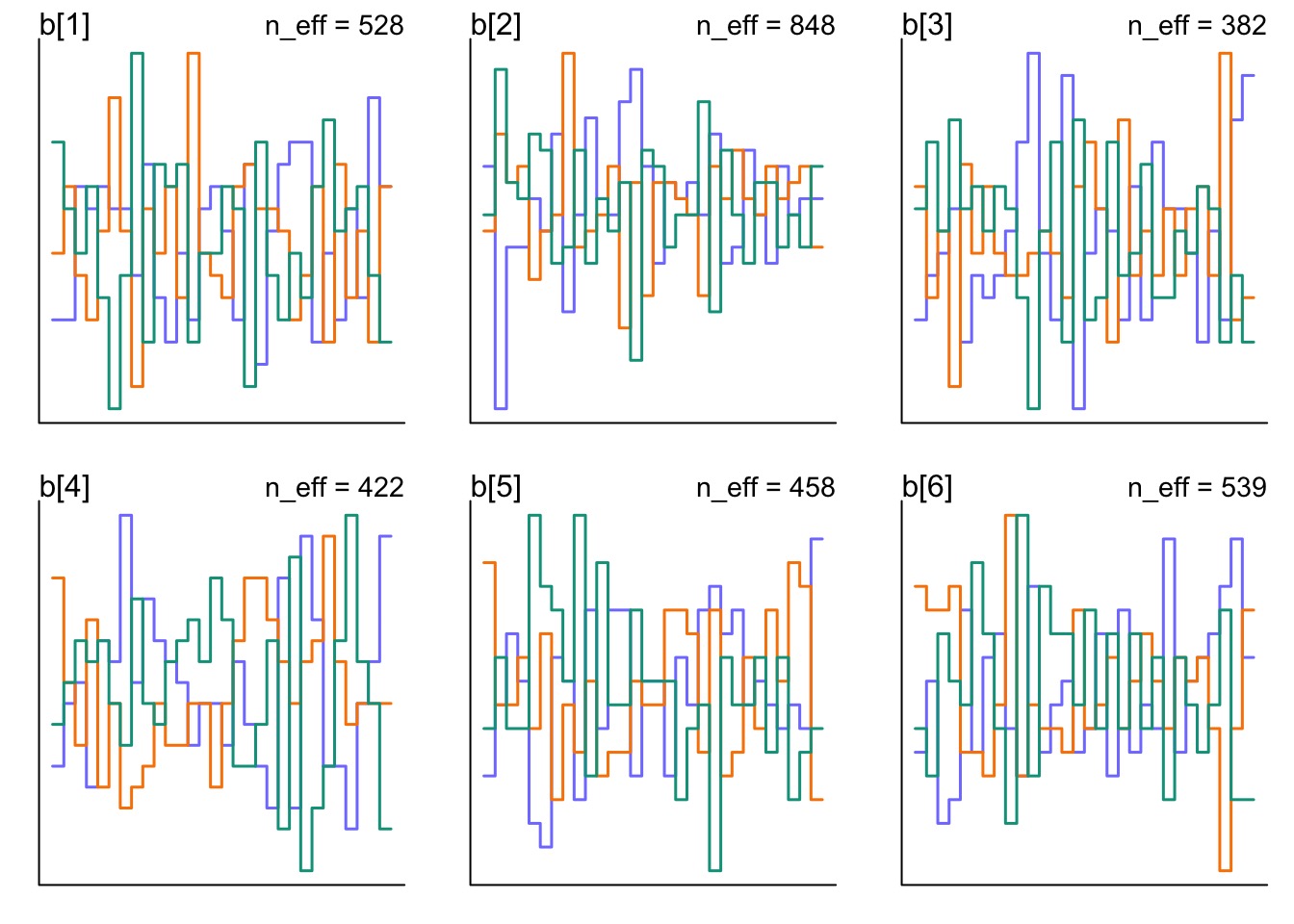
How is Z Mixing?

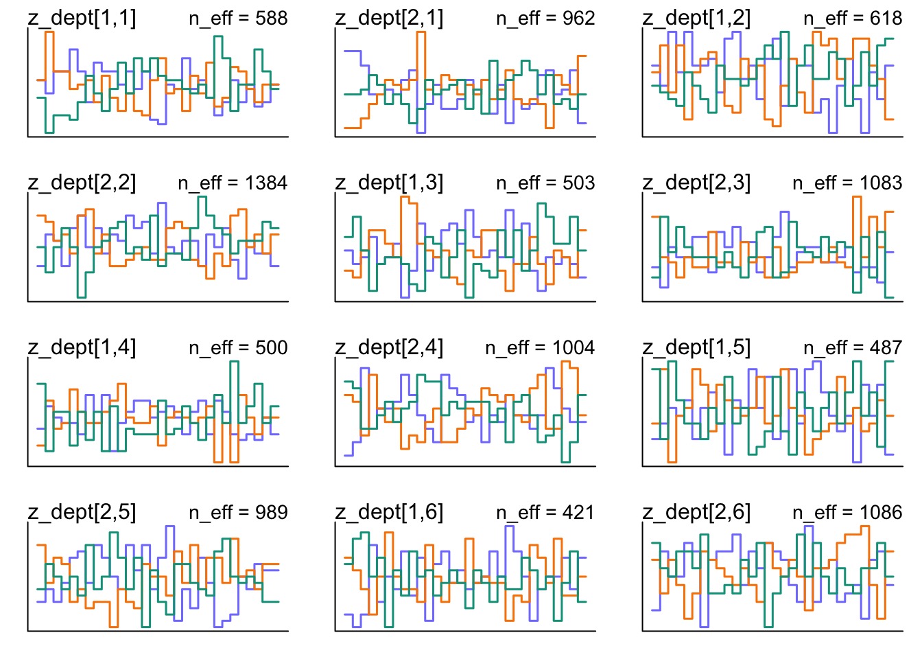
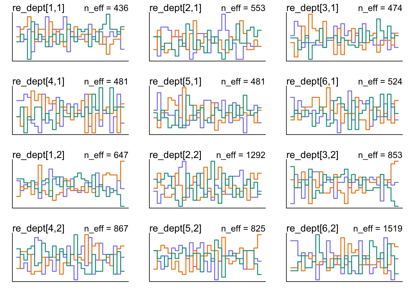
But how are our REs Mixing?

More transpars for easier comparison

mod_gender_dept_nc <- alist(
  #likelihood
  admit ~ dbinom(applications, p),
  
  #Data generating process
  logit(p) <- a_hat + a[dept_id] + b_hat*isMale + b[dept_id]*isMale,
  
  
  # NCP RE
  
  transpars > vector[6]:a <<- re_dept[,1],
  transpars > vector[6]:b <<- re_dept[,2],
  
  transpars > matrix[6, 2]:re_dept <- 
    compose_noncentered(sigma_dept, Rho_dept, z_dept),


  #priors
  a_hat ~ dnorm(0,10),
  b_hat ~ dnorm(0,10),
  
  # NCP priors
  matrix[2,6]:z_dept ~ normal( 0 , 1 ),
  vector[2]:sigma_dept ~ dexp(2),
  cholesky_factor_corr[2]:Rho_dept ~ lkj_corr_cholesky( 2 ),
  
  # convert Cholesky to Corr matrix
  gq> matrix[2,2]:Rho <<- Chol_to_Corr(Rho_dept)
)

Are they different?

NC

            mean        sd        5.5%      94.5%     rhat  ess_bulk
b[1] -0.55390227 0.2942779 -1.03078600 -0.1178819 1.004485  844.8861
b[2] -0.03935680 0.3068819 -0.50585594  0.4384510 1.001113 1095.9337
b[3]  0.24361848 0.2339808 -0.07225857  0.6379051 1.002734  674.7744
b[4]  0.07993483 0.2299250 -0.25628297  0.4473322 1.004246  646.0574
b[5]  0.28029734 0.2534287 -0.07537584  0.6841122 1.001586  824.2421
b[6]  0.06005412 0.2772689 -0.37816329  0.5132305 1.001427 1107.7910


Standard

            mean        sd       5.5%      94.5%     rhat ess_bulk
b[1] -0.57294559 0.3108684 -1.0762455 -0.1180378 1.002917 527.9177
b[2] -0.03393095 0.3227156 -0.5333867  0.4788650 1.000409 847.7560
b[3]  0.23581446 0.2536752 -0.1085711  0.6578231 1.001227 382.4475
b[4]  0.07157166 0.2518730 -0.2846817  0.4912321 1.001193 422.2788
b[5]  0.27099108 0.2730831 -0.1201936  0.7649616 1.002690 457.6668
b[6]  0.04700444 0.3192950 -0.4387460  0.5800213 1.002322 539.3690

Visualizing Random Effects

Viz of models with varying effects is tricky
WHAT IS YOUR QUESTION?
We often want only averages
But, we might want to incorporate our REs for future prediction

Dinosaur Allometry!

First, a model!

Dinosaurs$age_c <- Dinosaurs$age - mean(Dinosaurs$age)
Dinosaurs$log_mass <- log(Dinosaurs$mass)

Likelihood: \(log\ mass_i \sim N(\mu_i, \sigma)\)

DGP: \(\mu_i = \bar{a} + a_{species} + \bar{b} age\ centered_i + b_{species} age\ centered_i\)

RE: \([a_{species}, b_{species}] \sim MVN([0,0], R, [\sigma_a, \sigma_b])\)

Code it

dino_mod <- alist(
  
  # Likelihood
  
  # DGP
  
  # Varying Effects using NCP
  
  # Priors
  
  # NCP Priors for Varying Effects
  
)

Code it for 6 Species

dino_mod <- alist(
  
  # Likelihood
  log_mass ~ dnorm(mu, sigma),
  
  # DGP
  mu <- a_bar + a[sp_id] + b_bar * age_c + b[sp_id]* age_c,
  
  # Varying Effects using NCP
  transpars > vector[6]:a <<- re_mat[,1],
  transpars > vector[6]:b <<- re_mat[,2],
  
  transpars > matrix[6, 2]:re_mat <- 
    compose_noncentered(sigma_re, Rho_chol, z),


  #priors
  a_bar ~ dnorm(0,2),
  b_bar ~ dnorm(0,2),
  sigma ~ dexp(2),
  
  # NCP Priors for Varying Effects
  matrix[2,6]:z ~ normal( 0 , 1 ),
  vector[2]:sigma_re ~ dexp(2),
  cholesky_factor_corr[2]:Rho_chol ~ lkj_corr_cholesky( 2 ),
  
  # convert Cholesky to Corr matrix
  gq> matrix[2,2]:Rho <<- Chol_to_Corr(Rho_chol)
 
)

Fit!

dat <- Dinosaurs |>
  select(log_mass, age, age_c, sp_id, species)

dino_fit <- ulam(dino_mod,
                 dat,
                 chains = 3)

How did it do?

Coefficients and Predictions for Individual Species

dino_coefs <- tidy_draws(dino_fit)

dat_pred <- tibble(age = seq(1,15, length.out=100),
                       age_c = age - mean(dat$age)) |>
  crossing(sp_id = unique(dat$sp_id))

fit_pred <- linpred_draws(object = dino_fit, 
                          newdata = dat_pred)

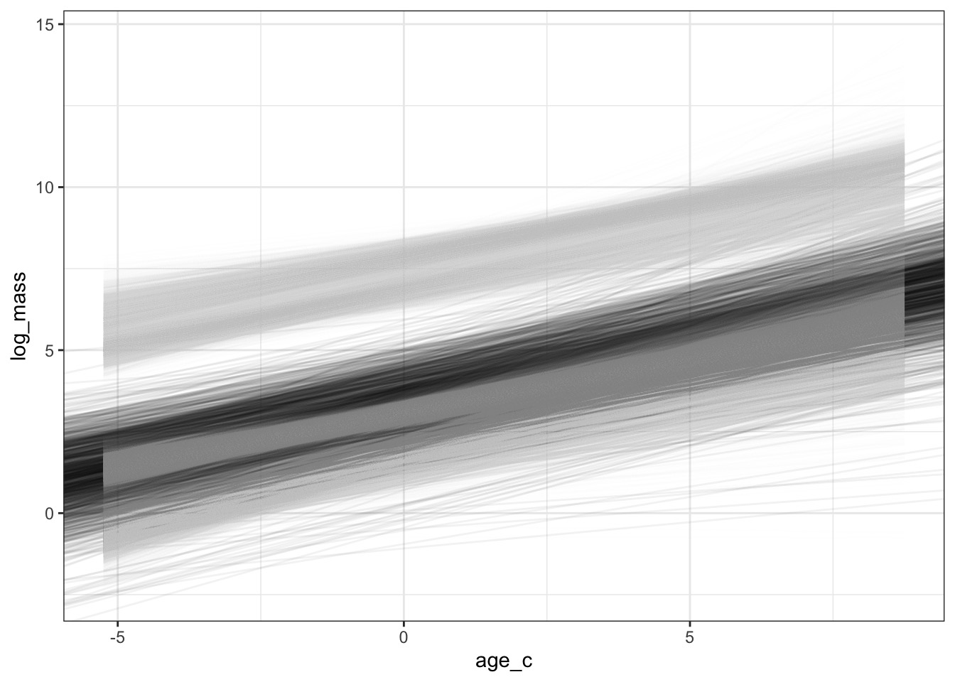
The Average Fit with Coefficient Uncertainty Only

With Each Species

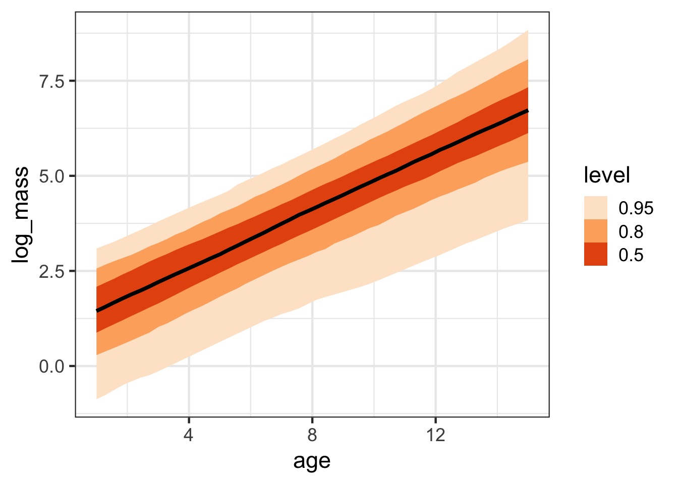
Or Credible Interval

crossing(
  tibble(age = seq(1,15, length.out=50),
                       age_c = age - mean(dat$age)),
  dino_coefs[1:500,]
) |>
  mutate(log_mass = a_bar + b_bar*age_c) |>
  ggplot(aes(x = age, y = log_mass)) +
  stat_lineribbon() +
  scale_fill_brewer(palette = "Oranges")

Or Credible Interval

With Each Species

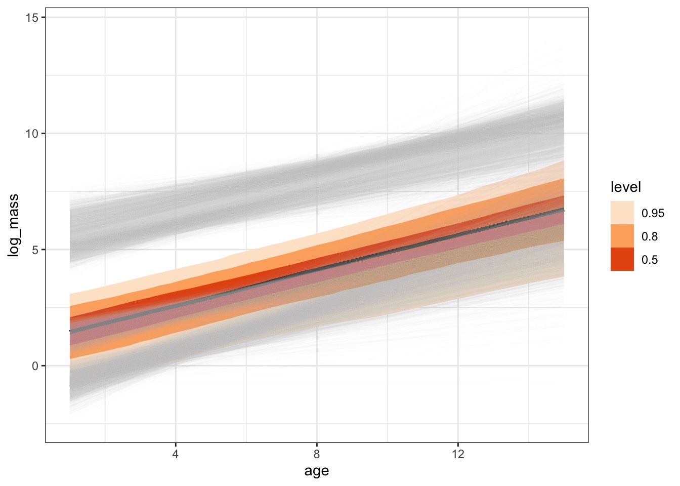
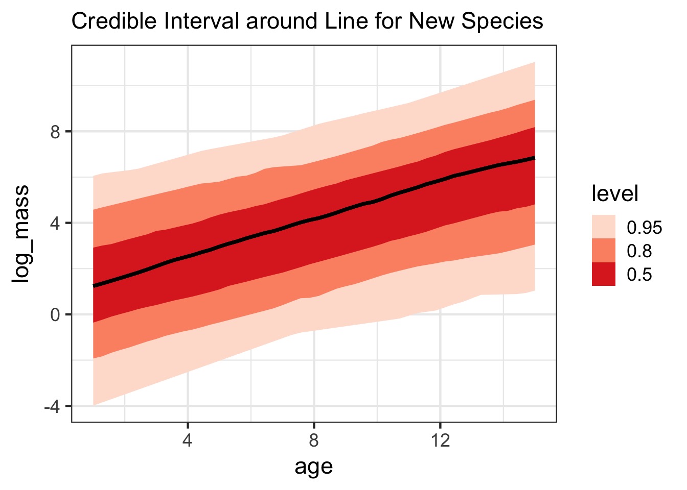
But What About New Species?

new_sp <- dino_coefs |>
  select(.draw, a_bar, b_bar, `sigma_re[1]`, `sigma_re[2]`, `Rho[1,2]`) |>
  group_by(.draw) |>
  reframe(re = rmvnorm2(1, 
                        sigma = c(`sigma_re[1]`, `sigma_re[2]`), 
                       Rho = matrix(c(1, `Rho[1,2]`, `Rho[1,2]`, 1), 
                                    ncol = 2)),
          a_bar = a_bar, 
          b_bar = b_bar) |>
  mutate(intercept = re[,1] + a_bar,
         slope = re[,2] + b_bar,
         )

But What About New Species?

Varying Slopes in Bayesian Mixed (aka Hierarchical, aka Multilevel) Models

Gender Discrimination in Graduate Admissions

Our data: Berkeley

A Poor First Model

How does it look?

What is the model we want?

What about this?

Notice how Slope and Intercept covary

Notice how Slope and Intercept covary

Dealing with Slope-Intercept Covariance

Building a Covariance Matrix with Correlations

Priors and Correlations

LKJ Correlation Distribution

So, those random effects…

A Variable Slope Intercept Model

What is new

Fitting

Did it blend?

Did it blend?

Did it blend?

Posterior Check

How correlated were slope and intercept?

How correlated were slope and intercept?

How correlated were slope and intercept?

How important was incorporating a random slope?

Density of Sigmas

Variable Intercept Only Model

Not quite as good of a fit…

WAIC suggests Variable Slope model better…

Optimization and Alternate Parameterization

Non-Centered Parameterization

Implications of Non-Centered Parameterization with Mixed Models

NC Paramterized Model

What is going on in this model matrices

Our NCP RE Matrix

Our Z-Scored Hyperprior

Our Hyperprior for Departmental Variances

Our Correlation Matrix

And let’s fit!

How is Z Mixing?

But how are our REs Mixing?

More transpars for easier comparison

Are they different?

Are they different?

Visualizing Random Effects

Dinosaur Allometry!

First, a model!

Code it

Code it for 6 Species

Fit!

How did it do?

How did it do?

Coefficients and Predictions for Individual Species

The Average Fit with Coefficient Uncertainty Only

With Each Species

Or Credible Interval

Or Credible Interval

With Each Species

But What About New Species?

But What About New Species?

Or Show with Credibility