Generalized Additive Models

Outline

1. Smoothing
   
   
2. GAMS and Basis Functions
   
   
3. Evaluating your GAM
   
   
4. GAMs, Space, Time

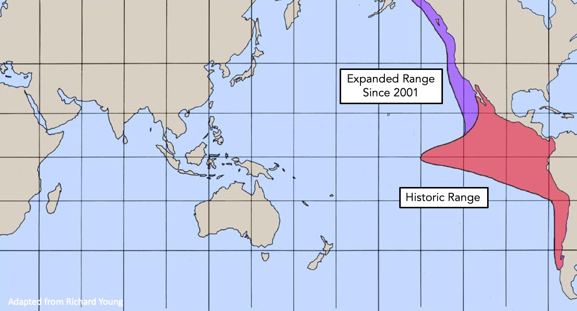
Humboldt Squid data from Julie Stewart Lowndes

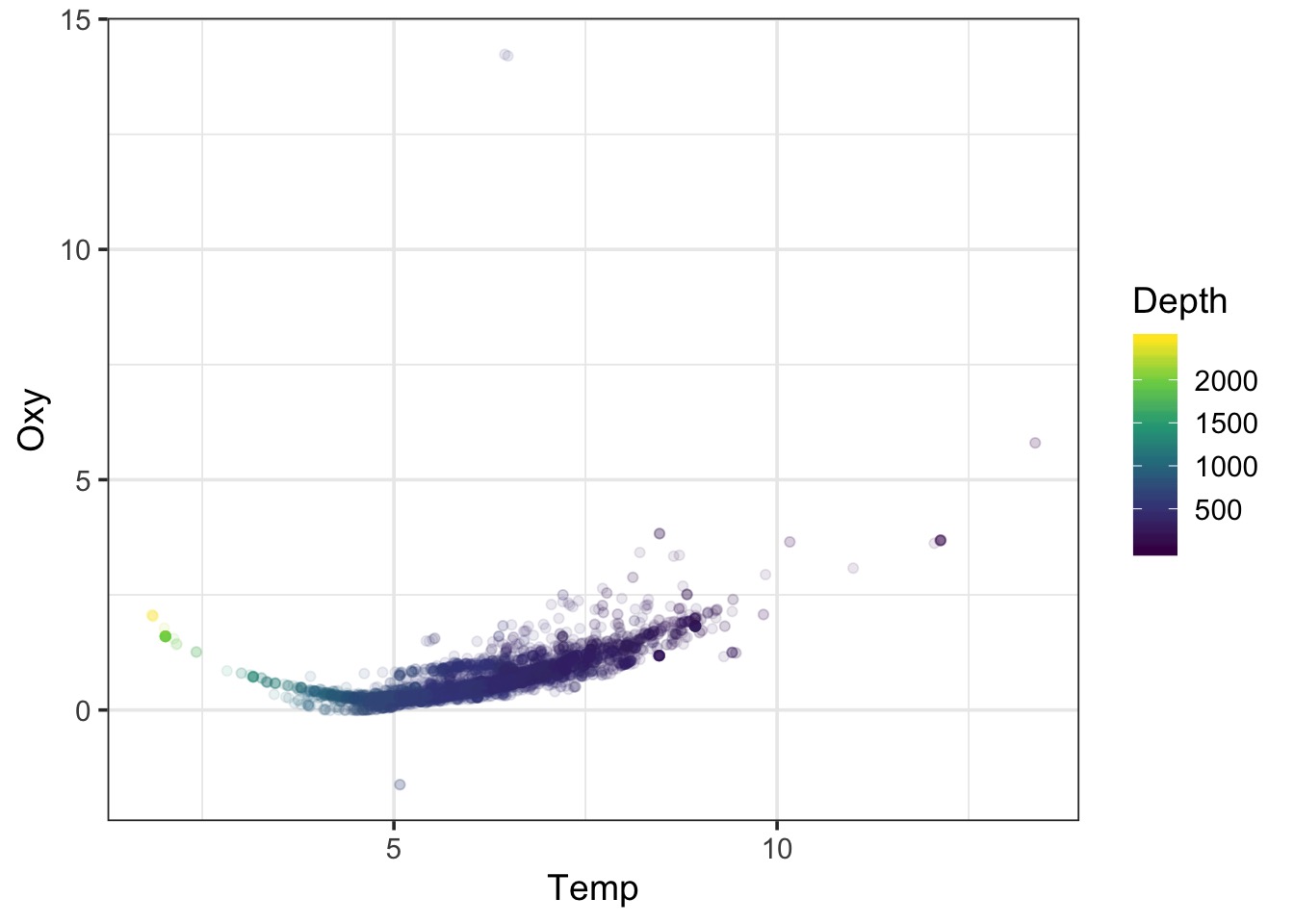
A Wiggly Problem: Temperature and Oxygen in Seawater Vertical Profiles

A Linear Fit

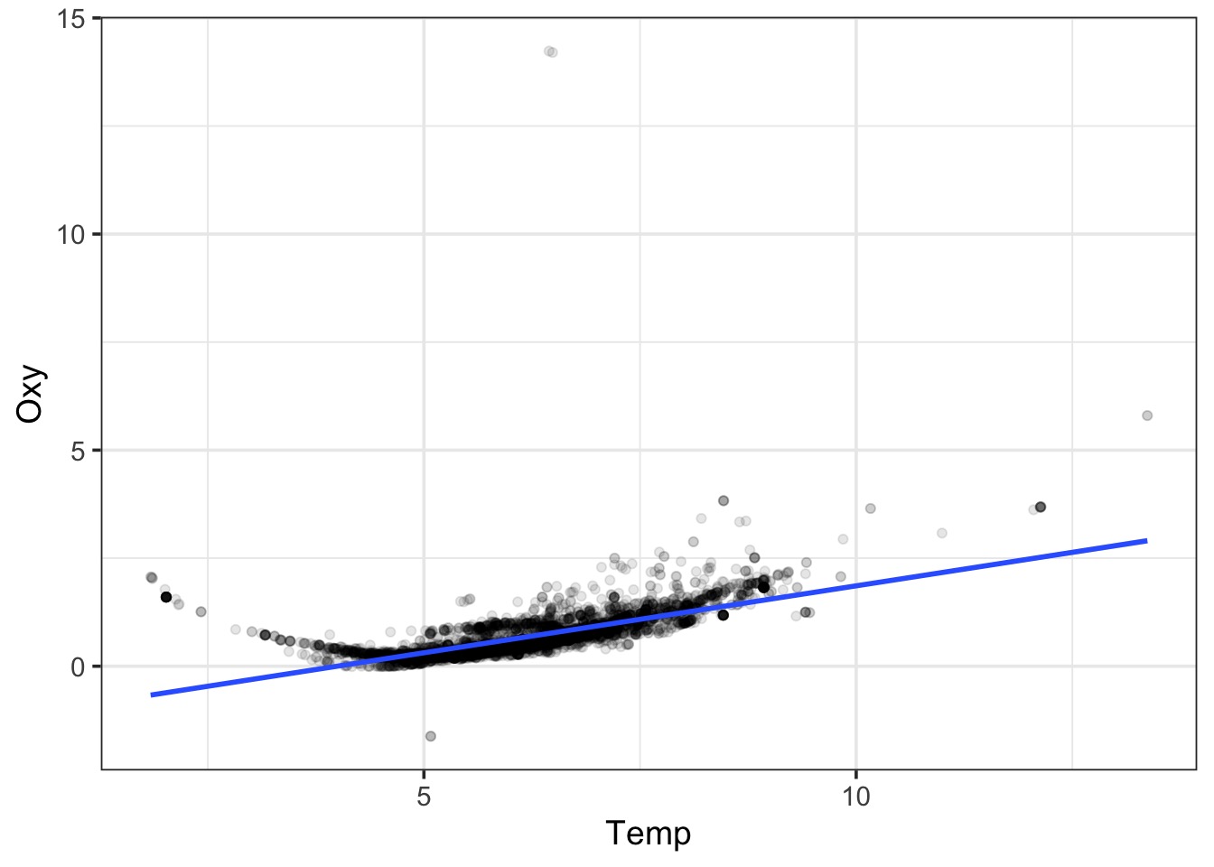
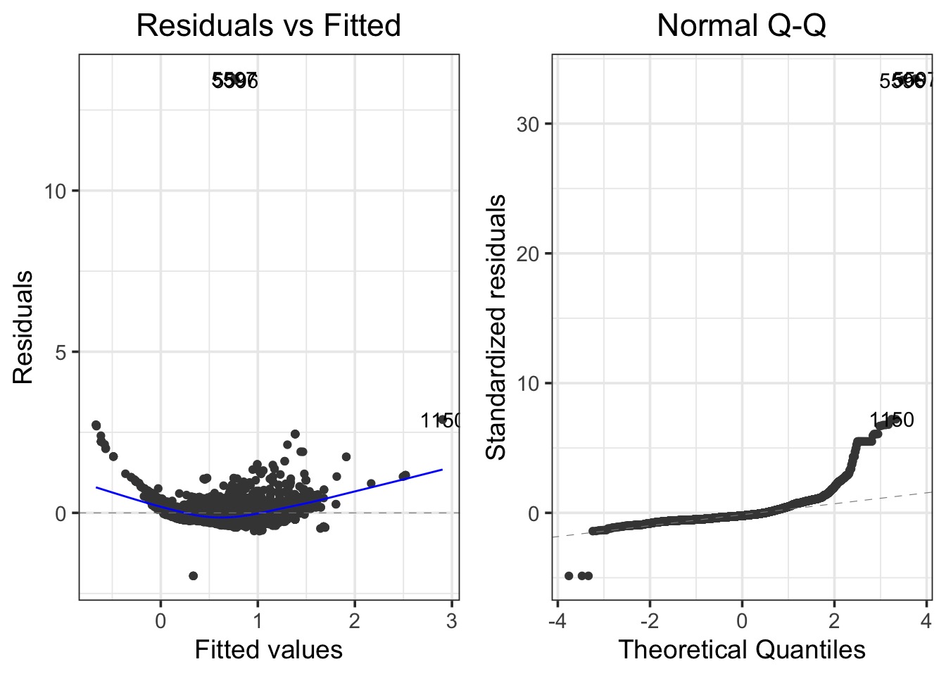
Bad Diagnostics!

What about a Polynomial?

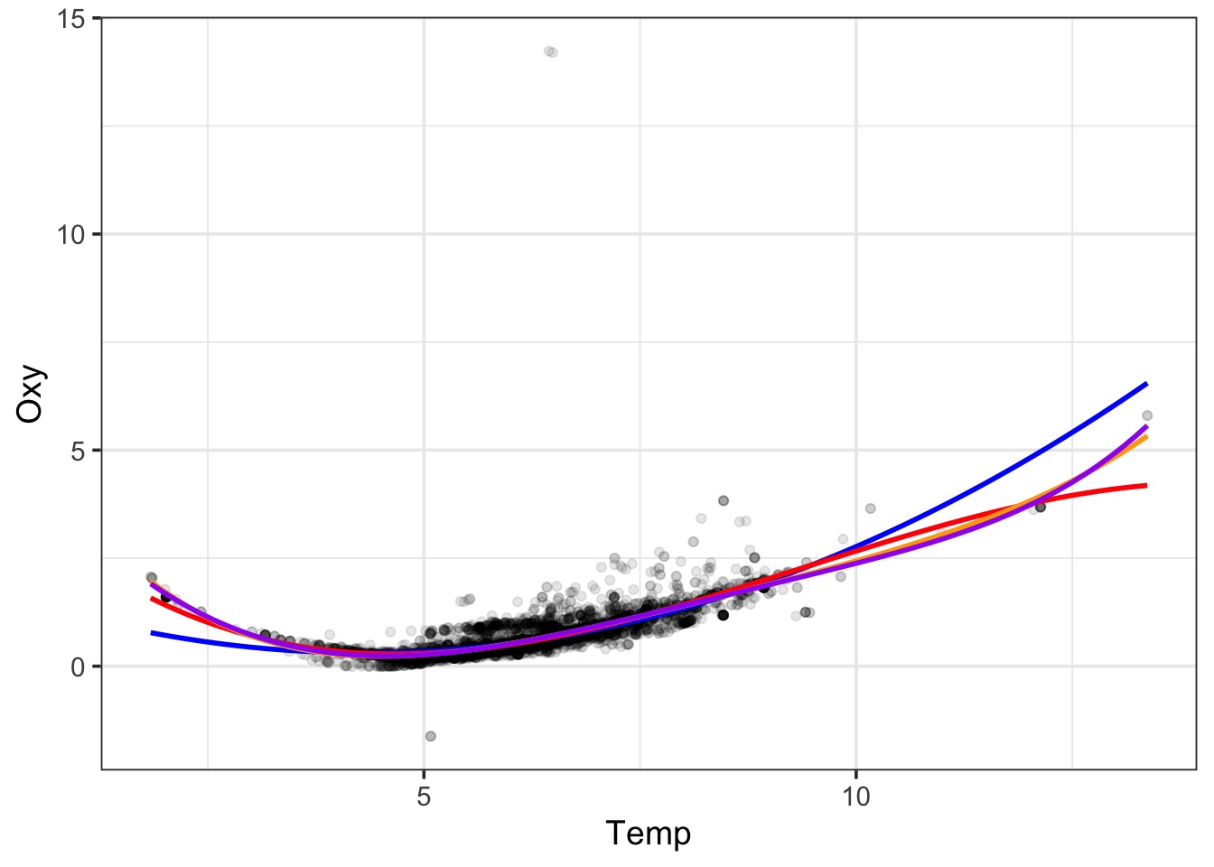
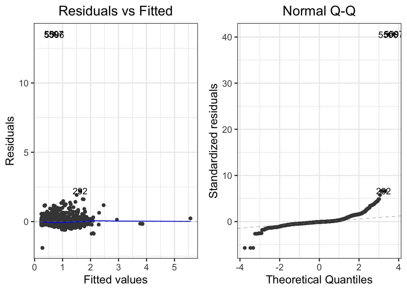
Bad Diagnostics, even at the 5th order!

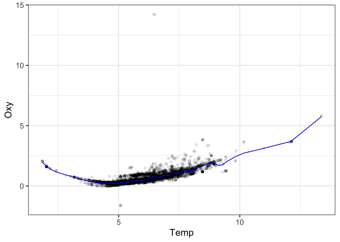
LOESS

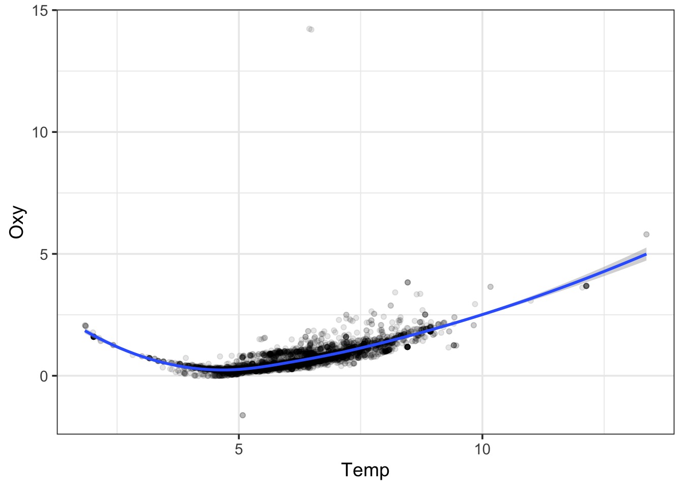
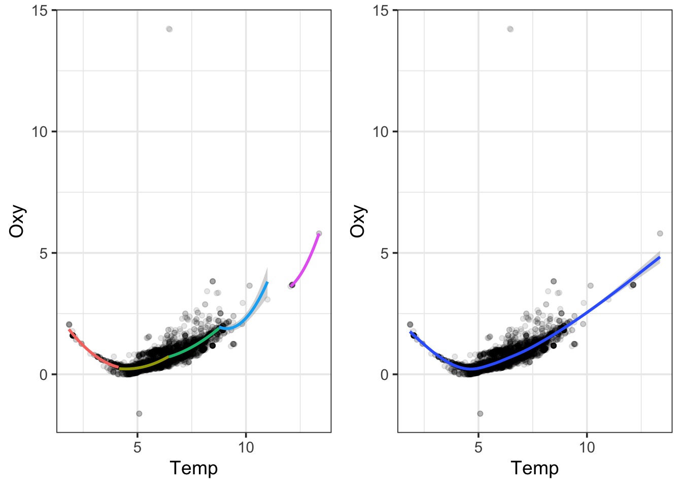
LOESS Takes Chunks

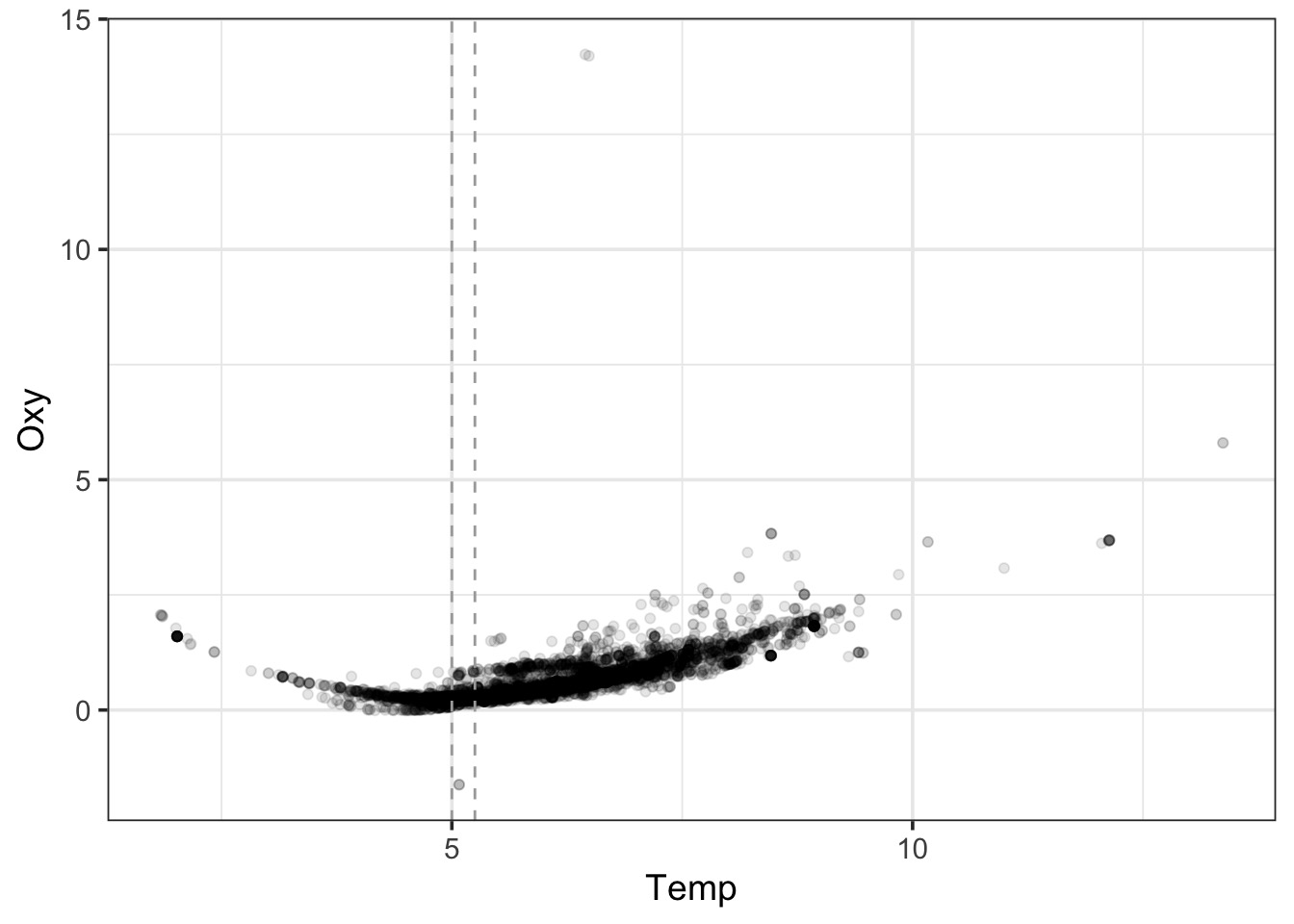
LOESS Takes Chunks

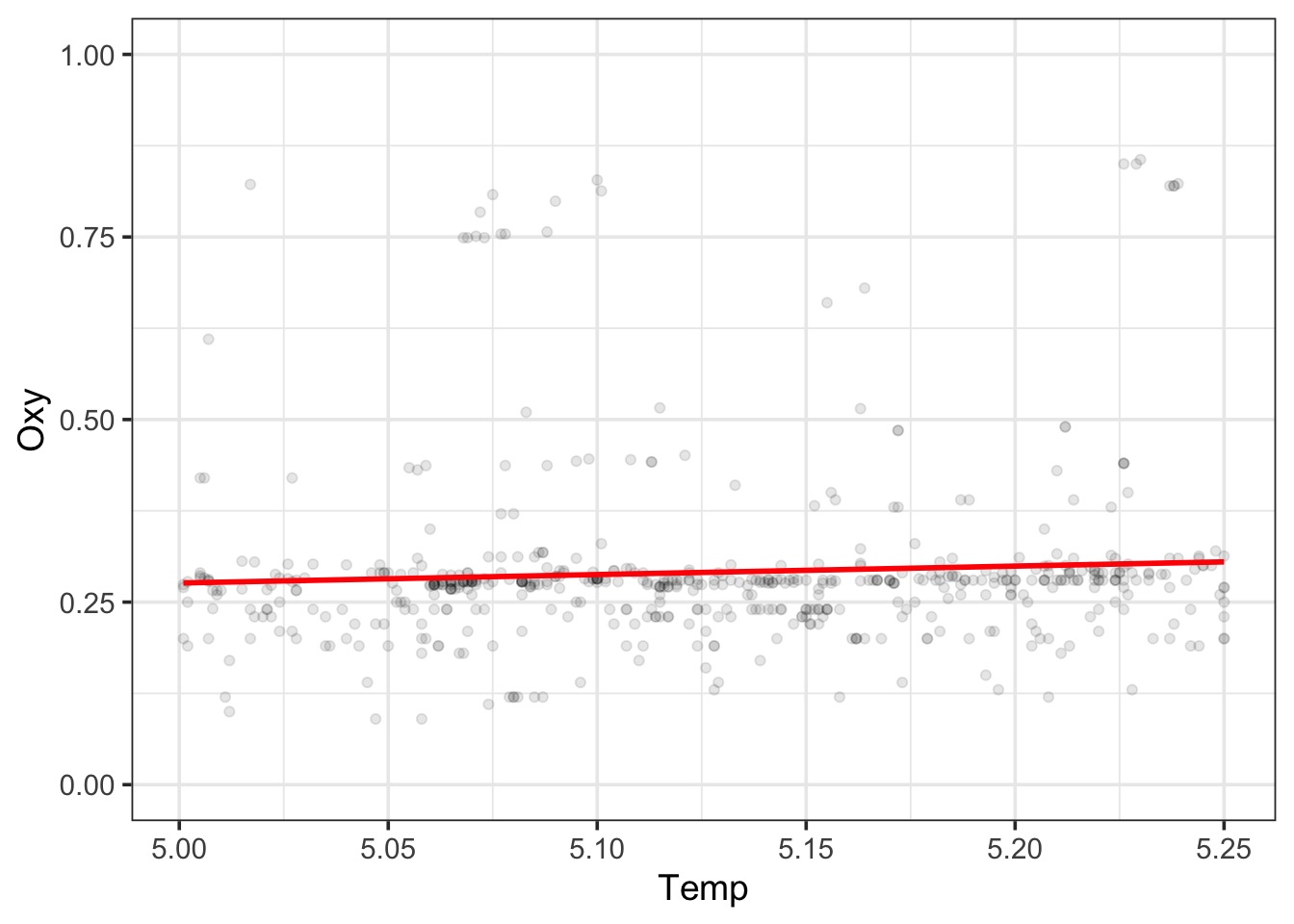
LOESS Takes Chunks

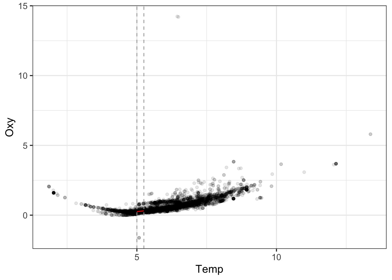
LOESS Takes Chunks

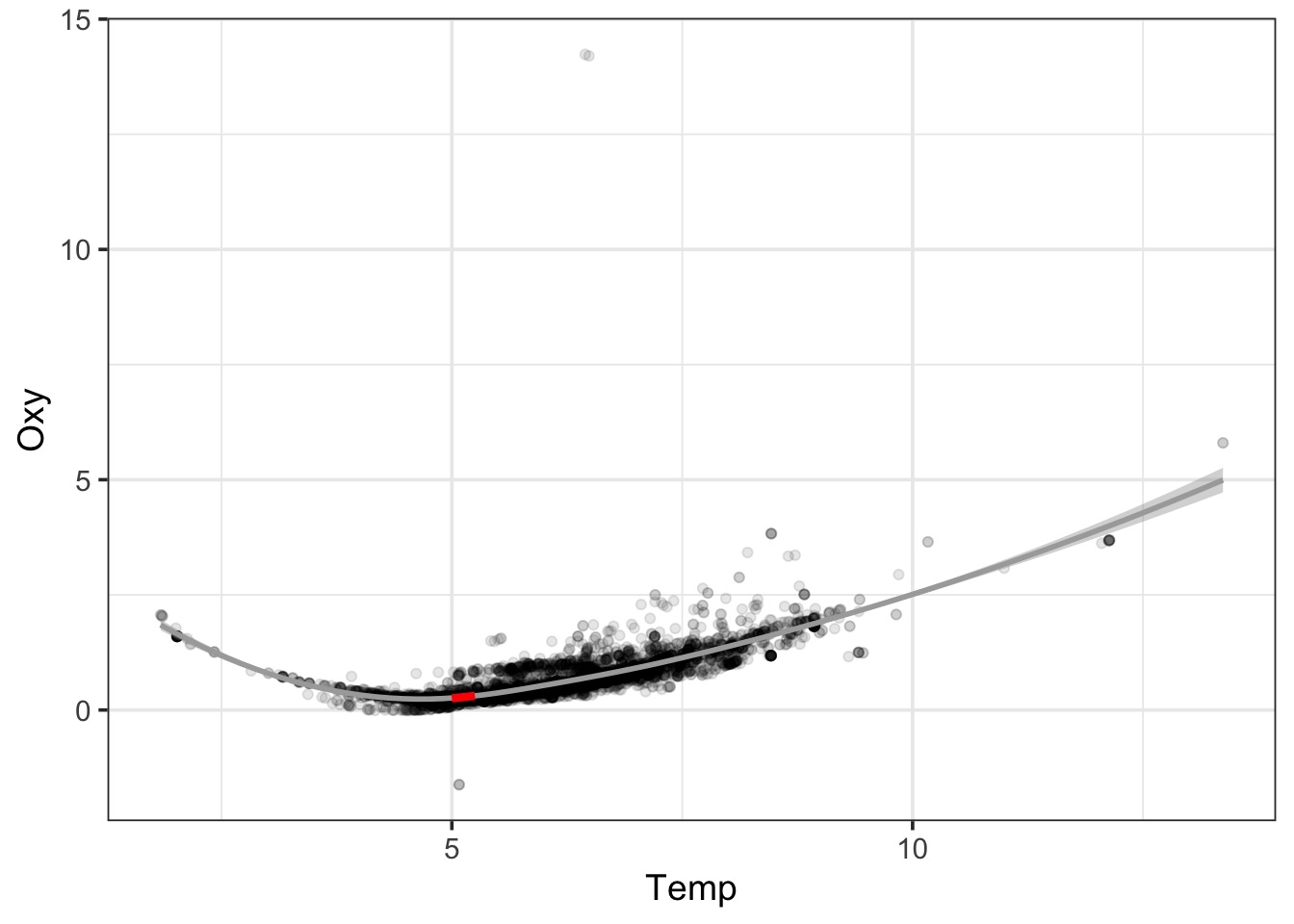
Smooth Splines Use Local Area Means

Problems with these techniques

• LM or GLM: We do not meet assumptions, and crazy residuals
  
  
• Polynomial: What polynomial to choose? Often misfit.
  
  
• LOESS: Not based on formula - purely phenomenological
  
  
• Splines: Just smoothed data. No real mechanism.

Outline

1. Smoothing
   
   
2. GAMS and Basis Functions
   
   
3. Evaluating your GAM
   
   
4. GAMs, Space, Time

The Central Idea Behind GAMs

• Standard Linear Model \[y\sim \mathcal{N}(\mu, \sigma^{2})\] \[\mu = b_{0}+b_{1}X_{1}\]
  
• Polynomial Regression \[y\sim \mathcal{N}(\mu, \sigma^{2})\] \[\mu = b_{0}+b_{1}X_{1}+b_{2}X^2\]
  
• GLM formulation \[y\sim \mathcal{N}(\mu, \sigma^{2})\] \[g(\mu) = b_{0}+b_{1}X_{1}+b_{2}X\]
  
• GAM formulation \[y\sim \mathcal{N}(\mu, \sigma^{2})\] \[g(\mu) = f(X)\]

The GAM Formulation in More Detail

\[y\sim \mathcal{N}(\mu, \sigma^{2})\]
\[g(\mu) = f(X)\]

\[ f(X) = \sum_{j=1}^{d}\gamma_jB_j(x)\]

The Cental Idea Behind GAMs

Basis Functions: You’ve seen them before

\[f(X) = \sum_{j=1}^{d}\gamma_jB_j(x)\]

Linear Regression as a Basis Function:
\[d = 1\]

\[B_j(x) = x\]

Basis Functions: You’ve seen them before

\[f(X) = \sum_{j=1}^{d}\gamma_jB_j(x)\]

Polynomial Regression as a Basis Function:
\[f(x) = \gamma_0 + \gamma_1\cdot x^1 \ldots +\gamma_d\cdot x^d\]

Basis Functions in GAMs

• You can think of every \(B_j(x)\) as a transformation of x
  
  
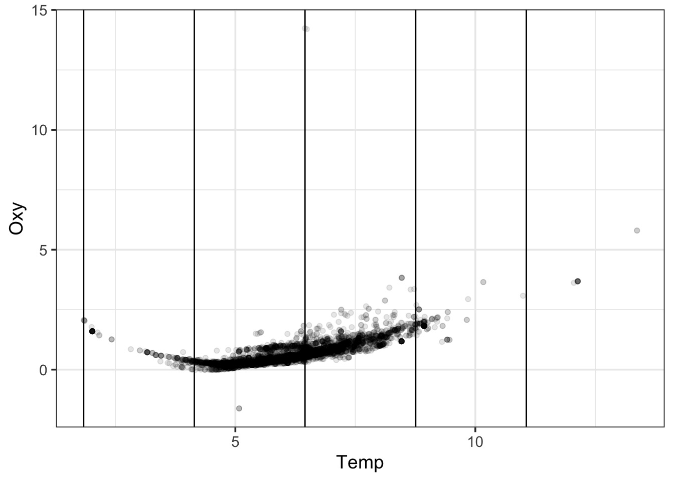
• In GAMs, we base j off of K knots
  
  
• A knot is a place where we split our data into pieces
  • We optimize knot choice, but let’s just split evenly for a demo
    
• For each segment of the data, we fit a seprate function, then add them together

Consider our data

Consider our data

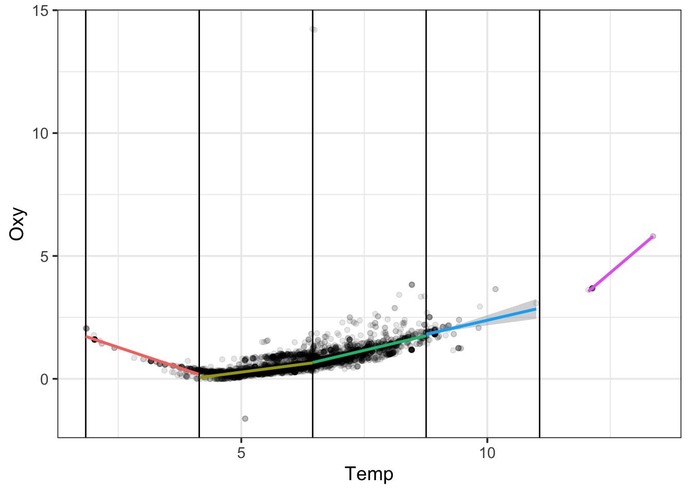
A Square Fit

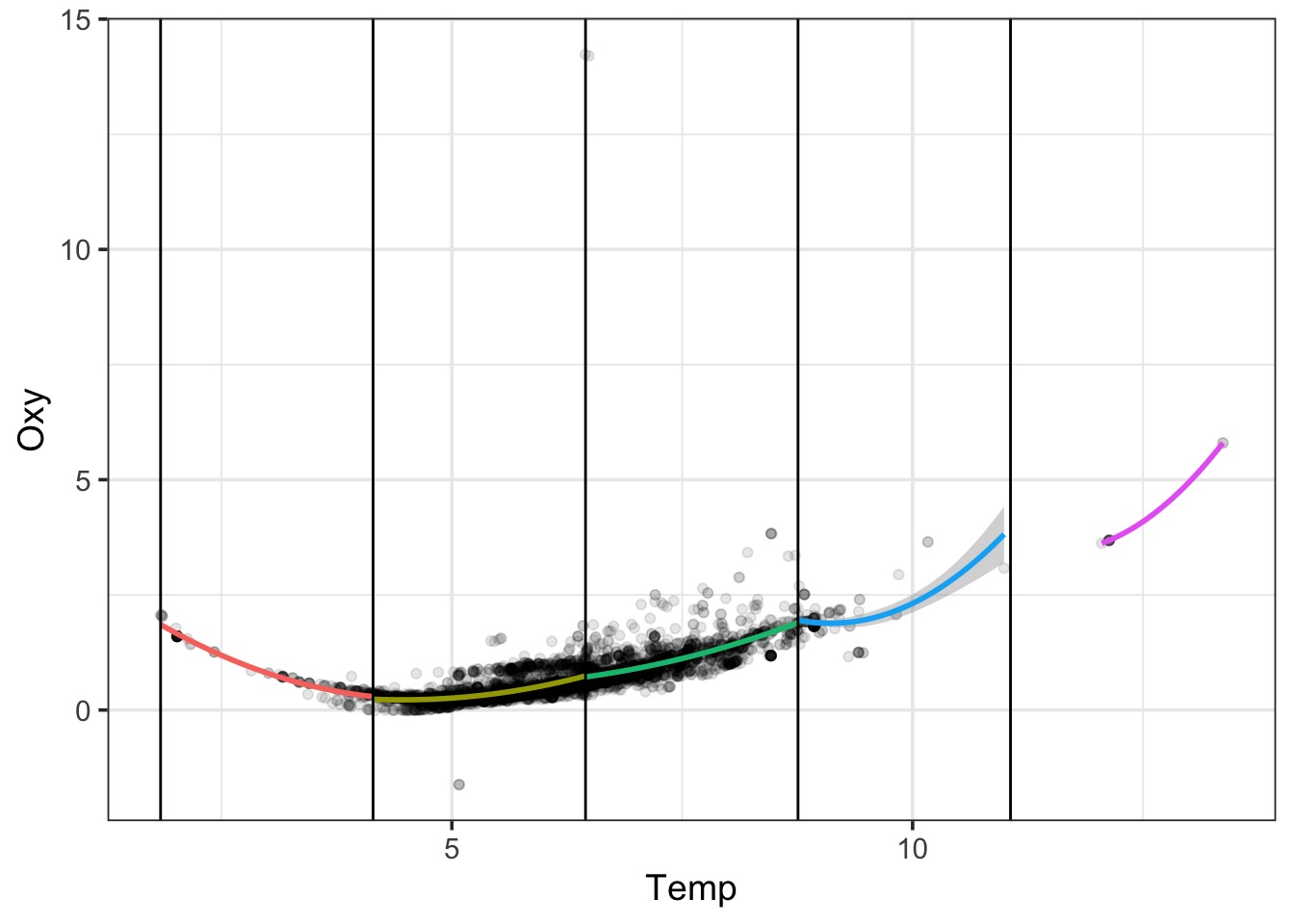
A Cubic GAM

How do we fit

• Use penalized likelihood
  \[l_p(\beta)= l(\beta) - \color{darkred}{\mathcal{penalty}}\]
  
  
• Penality adjust for ‘wiggliness’
  \[l_p(\beta)= l(\beta) - \color{#b2001d}{\lambda B'SB}\]
  
• S is a penalty matrix, and \(\lambda\)
  • \(\lambda\) = 2 by default, but play with it!

Fitting As a Gam

library(mgcv)

fit <- gam(Oxy ~ s(Temp, bs = "cr"), data = squid)

Many Different Kind of Basis Functions

• Thin Plate Regression Splines
  • bs = "tp"
    
  • Default
    
  • Analgous to looking at bending within each region of basis
    
    
• Cubic Regression
  • bs = "cr"
    
  • Raises (x-k) to up to the 3rd power
     
    ## Many Different Kind of Basis Functions
    
• Random Effects
  • bs = "re"
    
    
• P-Splines
  • bs = "ps"
    
  • Penalized B-spline
    
  • Flexible bands passing through several points

Interaction Effect Basis Functions via Tensor Products

• bs = "ts"
  • One set of penalties per marginal basis
    
    
• bs = "ti"
  • Excludes main effects
     
    
• bs = "t2"
  • One penalty set per term

GAMs and Causal Inference

• We are fitting something to a mean structure, not error
  
  
• More direct control of partial correlations
  
  
• BUT - estimating many terms for the basis
  
  
• So, more akin to mixed models
  
  
• Causal implications less clear than fixed effects

Outline

1. Smoothing
   
   
2. GAMS and Basis Functions
   
   
3. Evaluating your GAM
   
   
4. GAMs, Space, Time

Evaluating Assumptions

par(mfrow=c(2,2))
gam.check(fit,  k.rep=1000)

par(mfrow = c(1,1))

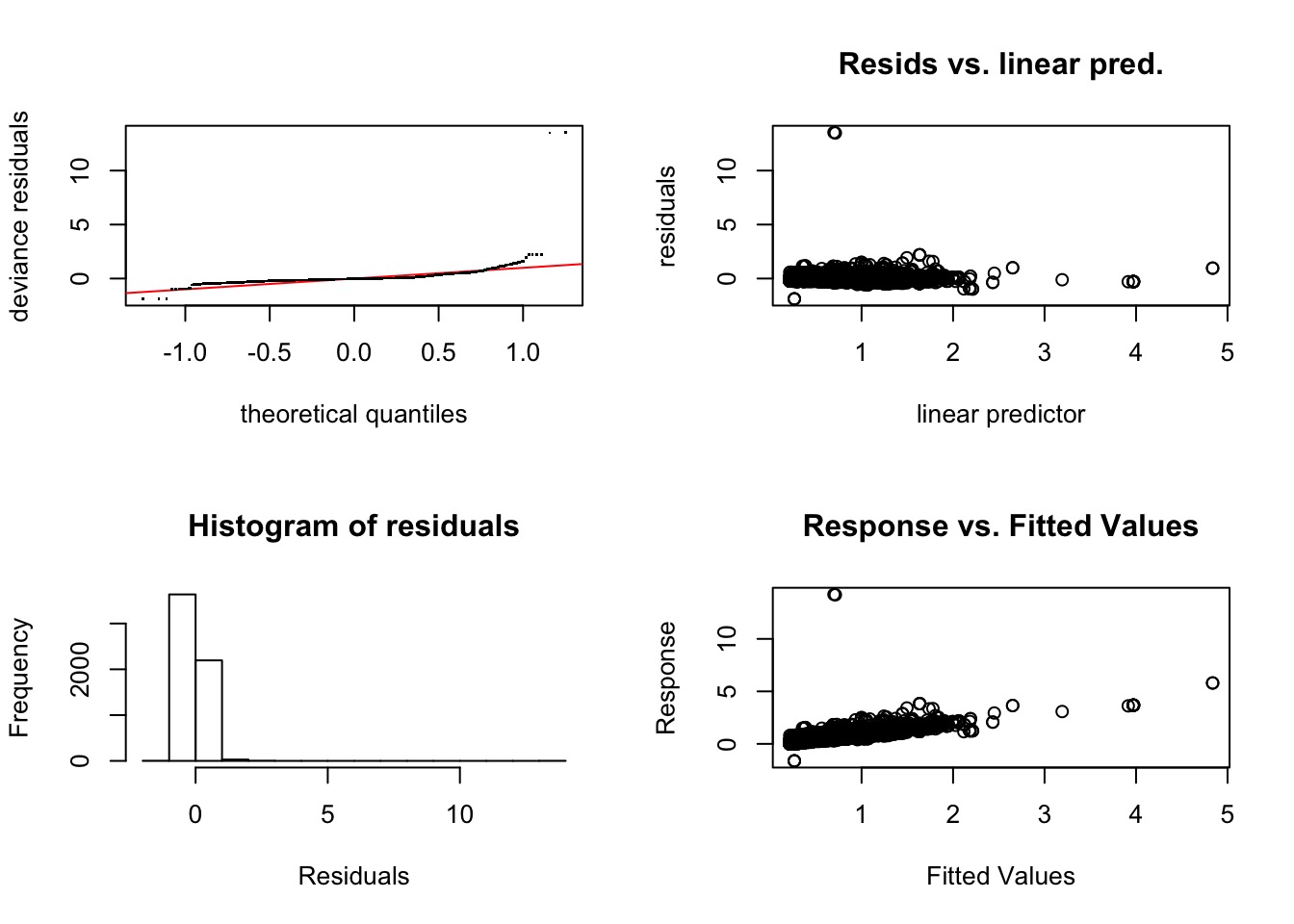
Evaluating Assumptions

>gam.check(fit,  k.rep=1000)

Method: GCV   Optimizer: magic
Smoothing parameter selection converged after 4 iterations.
The RMS GCV score gradient at convergence was 2.959763e-07 .
The Hessian was positive definite.
Model rank =  10 / 10 

Basis dimension (k) checking results. Low p-value (k-index<1) may
indicate that k is too low, especially if edf is close to k'.

          k'  edf k-index p-value    
s(Temp) 9.00 6.89    0.93   0.001 ***
---
Signif. codes:  0 ‘***’ 0.001 ‘**’ 0.01 ‘*’ 0.05 ‘.’ 0.1 ‘ ’ 1

Model Evaluation

Effective DF = DF adjusted for penalty

anova(fit)

Family: gaussian 
Link function: identity 

Formula:
Oxy ~ s(Temp, bs = "cr")

Approximate significance of smooth terms:
          edf Ref.df    F p-value
s(Temp) 6.888  7.726 1233  <2e-16

Assessing Fit

summary(fit)

Family: gaussian 
Link function: identity 

Formula:
Oxy ~ s(Temp, bs = "cr")

Parametric coefficients:
            Estimate Std. Error t value Pr(>|t|)    
(Intercept) 0.646192   0.004348   148.6   <2e-16 ***
---
Signif. codes:  0 '***' 0.001 '**' 0.01 '*' 0.05 '.' 0.1 ' ' 1

Approximate significance of smooth terms:
          edf Ref.df    F p-value    
s(Temp) 6.888  7.726 1233  <2e-16 ***
---
Signif. codes:  0 '***' 0.001 '**' 0.01 '*' 0.05 '.' 0.1 ' ' 1

R-sq.(adj) =  0.619   Deviance explained =   62%
GCV = 0.11108  Scale est. = 0.11093   n = 5868

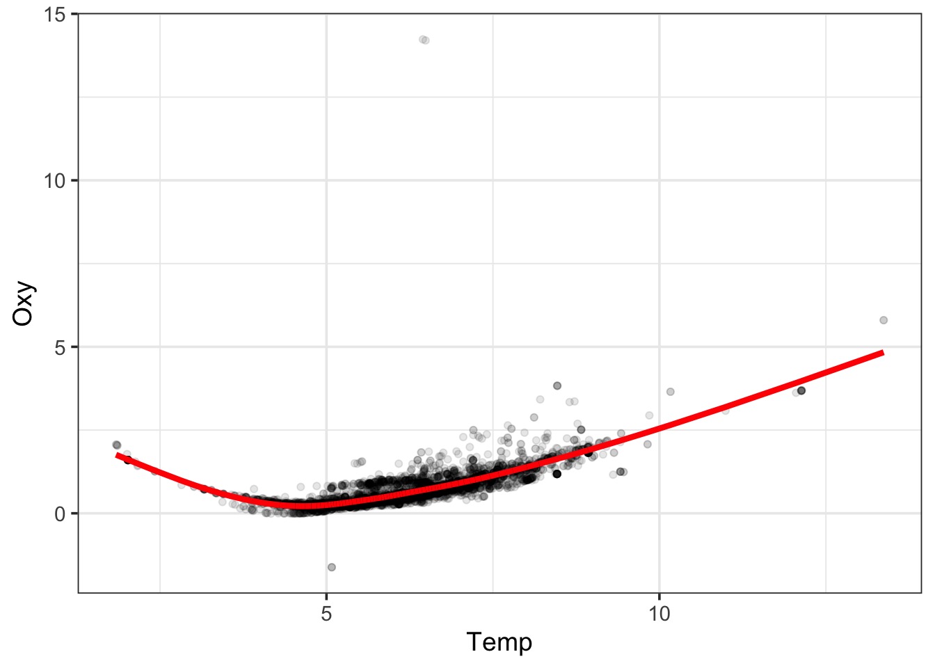
Visualizing

squid$pred <- predict(fit)

temp_oxy +
  geom_line(data = squid, mapping = aes(y = pred),
            color = "red", lwd = 1.5)

Visualizing

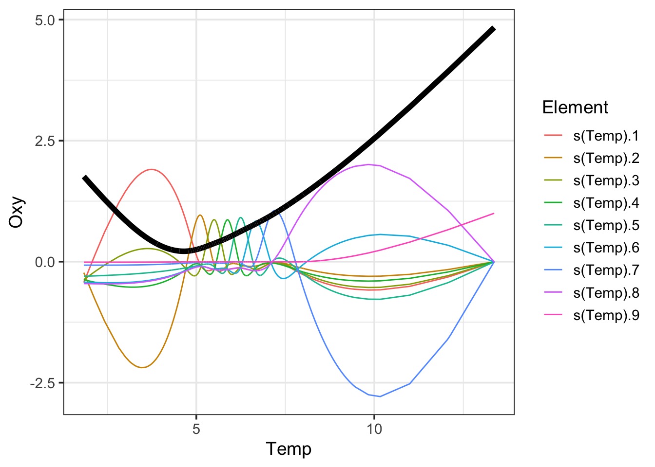
Peeking Inside the Black Box

predict(fit, type = "lpmatrix") %>%
  as_tibble()

# A tibble: 5,868 x 10
   `(Intercept)` `s(Temp).1` `s(Temp).2` `s(Temp).3` `s(Temp).4`
           <dbl>       <dbl>       <dbl>       <dbl>       <dbl>
 1             1     -0.0196     -0.0116     -0.0122     -0.0349
 2             1     -0.0196     -0.0116     -0.0122     -0.0349
 3             1     -0.165       0.0358      0.847      -0.217 
 4             1     -0.178      -0.0933     -0.155      -0.148 
 5             1     -0.130      -0.0651     -0.127      -0.0579
 6             1     -0.169      -0.0867     -0.154      -0.113 
 7             1     -0.169      -0.0871     -0.154      -0.115 
 8             1     -0.511      -0.264      -0.462      -0.361 
 9             1     -0.348      -0.181      -0.311      -0.263 
10             1     -0.315      -0.164      -0.280      -0.242 
# … with 5,858 more rows, and 5 more variables: `s(Temp).5` <dbl>,
#   `s(Temp).6` <dbl>, `s(Temp).7` <dbl>, `s(Temp).8` <dbl>,
#   `s(Temp).9` <dbl>

Visualizing the Black Box

Outline

1. Smoothing
   
   
2. GAMS and Basis Functions
   
   
3. Evaluating your GAM
   
   
4. GAMs, Space, Time

Basis Functions for Space and Time

• Gaussian Process
  • bs = "gp"
  • Can choose the model with mod = 1:5
    
  • An approximation, but close enough!
    
  • For point processes, time series, etc.
  • Models the mean
    
    
• Modeling error
  - Can use corAR1 or anything
  - Not causal
  
  
• Discrete places (e.g., polygons)
  • bs = 'mrf': Markov Random Field
  • Like SAR

Global Temperature Example

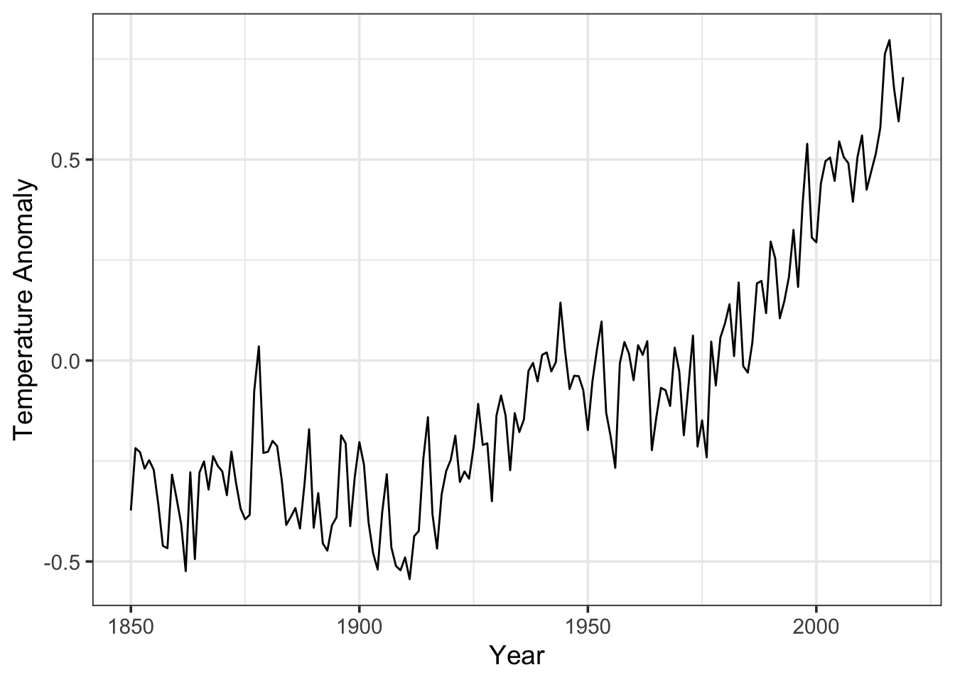
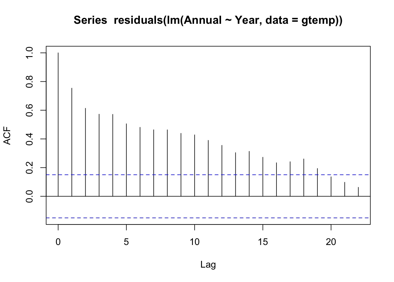
Any ACF from a Linear Fit?

acf(residuals(lm(Annual ~ Year, data = gtemp)))

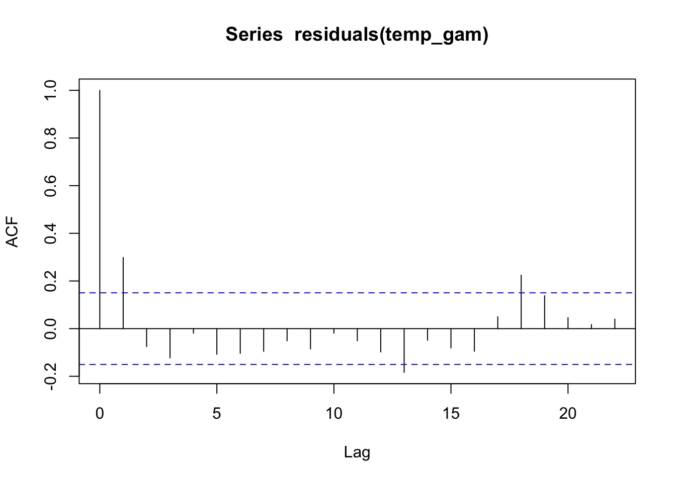
A GAM Timeseries Fit

temp_gam <- gam(Annual ~ s(Year, bs = "gp"), data = gtemp)

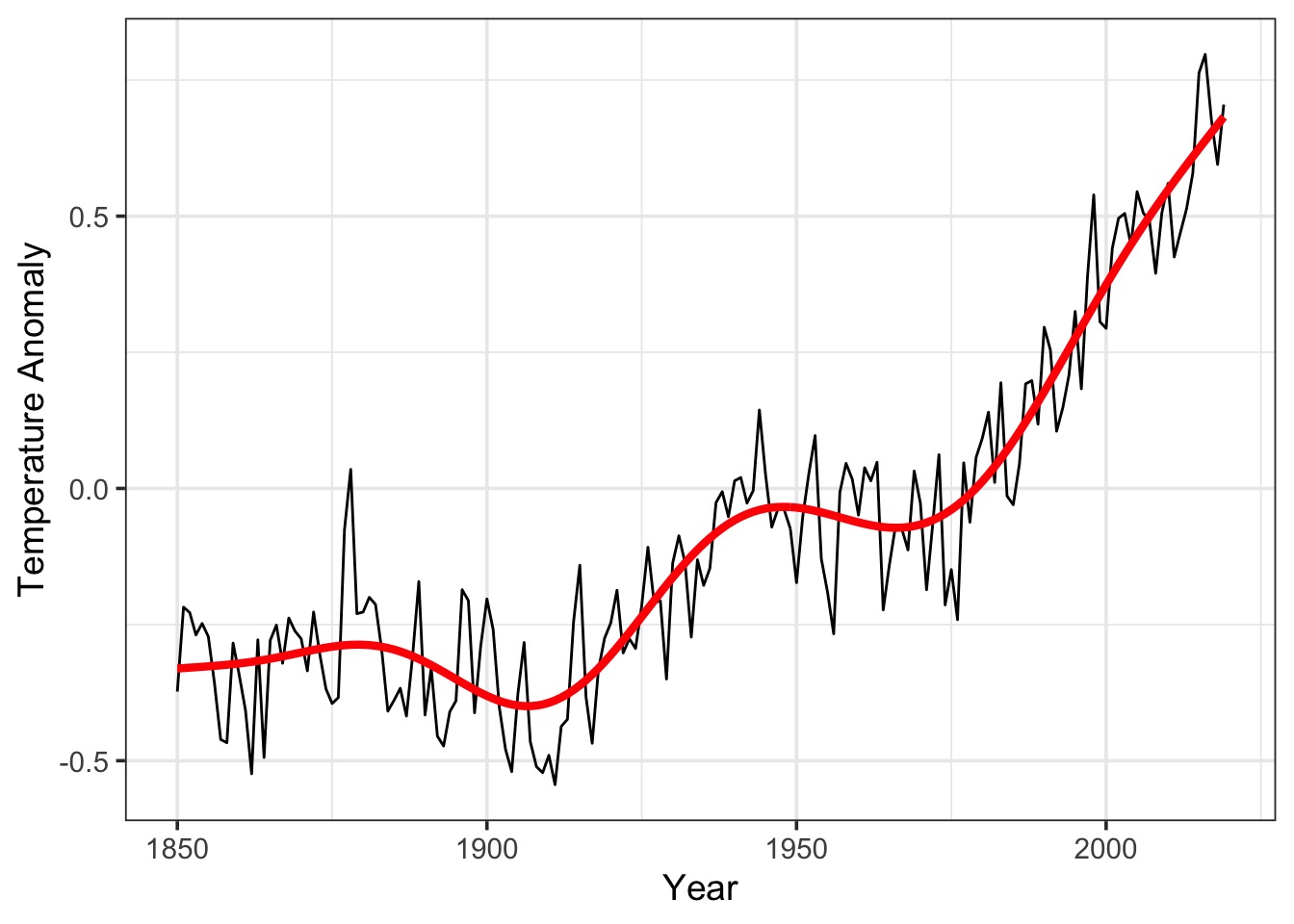
Did it Blend?

The Fit

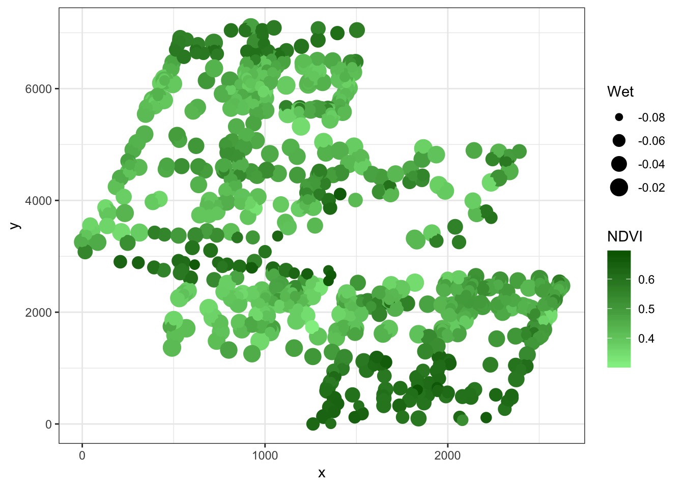
What about Space?

<ScaleContinuous>
 Range:  
 Limits:    0 --    1

But there are drivers

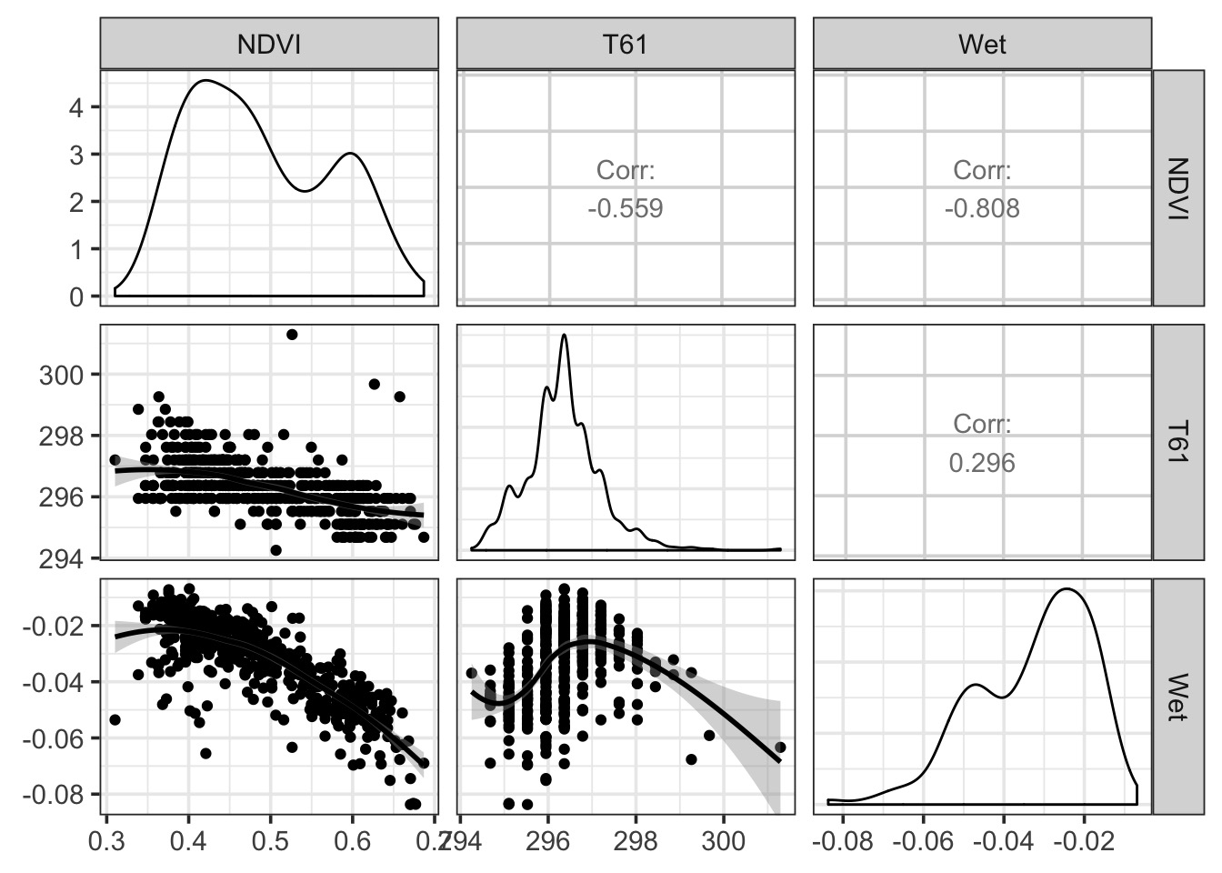
Naieve Analysis of Point Pattern Data with GAMs!

boreal_mod <- gam(NDVI ~ s(Wet) + s(T61), 
                  data = boreal)

But…spatial autocorrelation

library(gstat)
v_bor_resid <- variogram(residuals(boreal_mod) ~ 1, 
                         loc= ~x+y, data = boreal)
plot(v_bor_resid)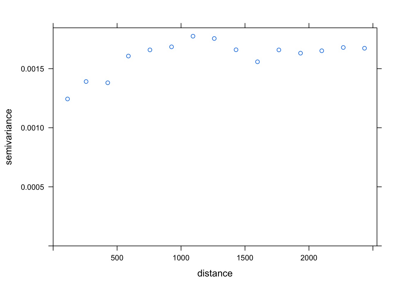

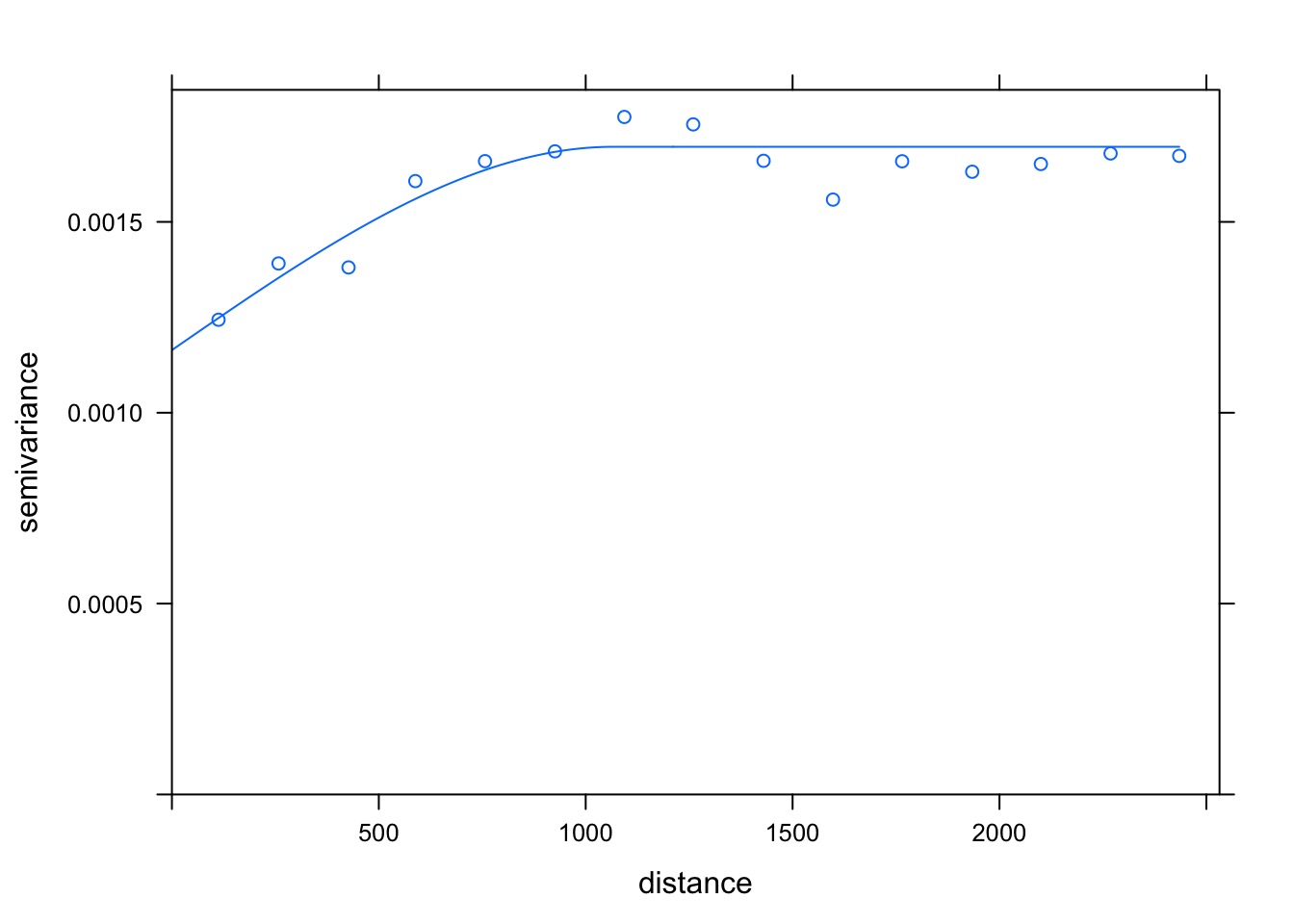
What’s the Shape?

best_resid_vario <- fit.variogram(v_bor_resid, 
              model = vgm(c("Gau", "Mat", "Sph")))

best_resid_vario

  model        psill    range
1   Nug 0.0011640961    0.000
2   Sph 0.0005326058 1066.352

Spherical Autocorrelation!

A Spatial GAM

boreal_mod_spatial <- gam(NDVI ~ s(Wet) + s(T61) +
                    s(x, y, bs = "gp", m = 1), 
                  data = boreal)

Did It Blend?

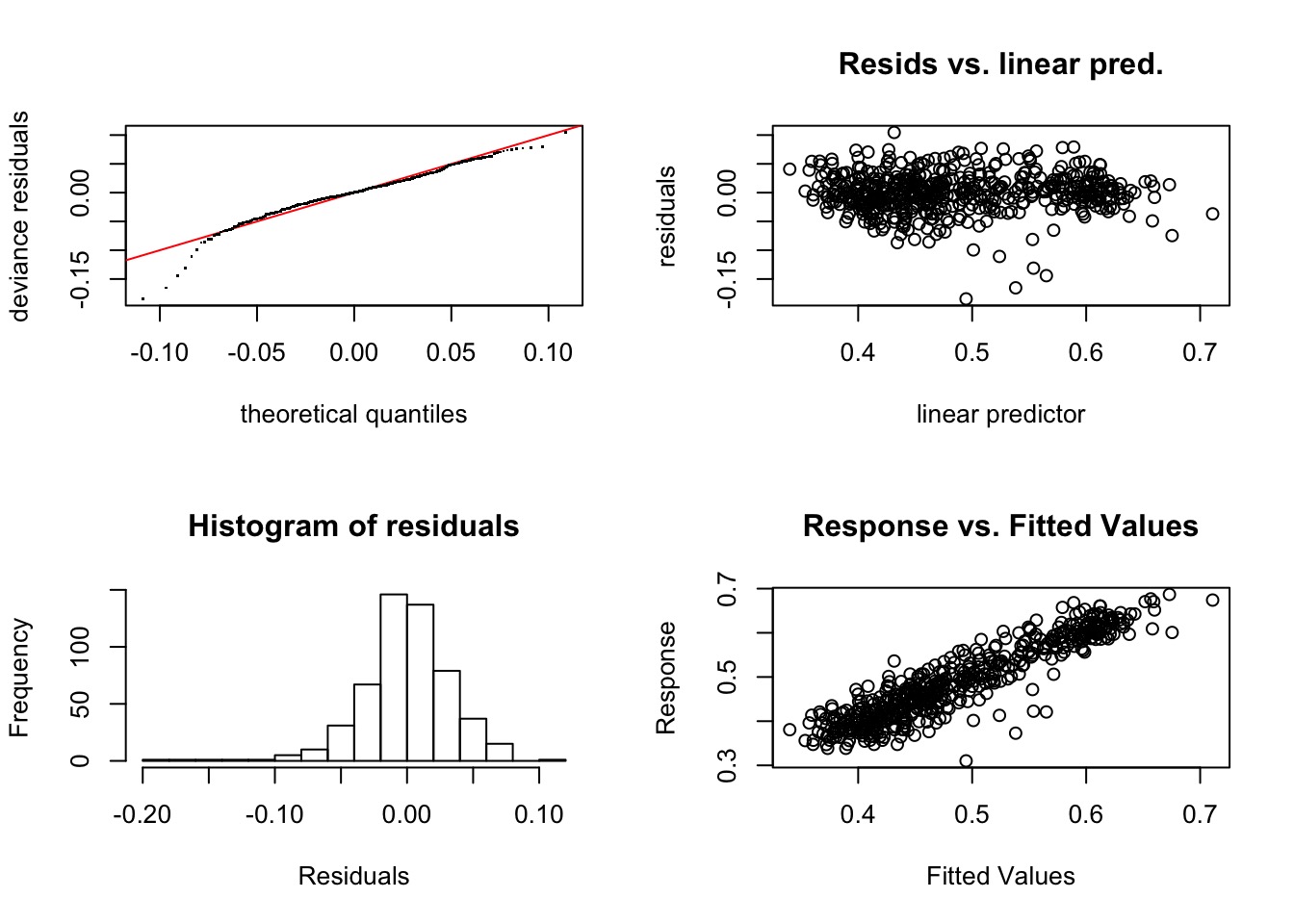
Method: GCV   Optimizer: magic
Smoothing parameter selection converged after 11 iterations.
The RMS GCV score gradient at convergence was 8.119027e-08 .
The Hessian was positive definite.
Model rank =  51 / 51 

Basis dimension (k) checking results. Low p-value (k-index<1) may
indicate that k is too low, especially if edf is close to k'.

          k'   edf k-index p-value    
s(Wet)  9.00  2.87    1.02    0.64    
s(T61)  9.00  8.54    0.89  <2e-16 ***
s(x,y) 32.00 22.83    0.83  <2e-16 ***
---
Signif. codes:  0 '***' 0.001 '**' 0.01 '*' 0.05 '.' 0.1 ' ' 1

Refit with Higher K for Space

boreal_mod_spatial <- gam(NDVI ~ s(Wet) + s(T61) +
                    s(x, y, bs = "gp", m = 1, k = 100), 
                  data = boreal)

Did It Blend?

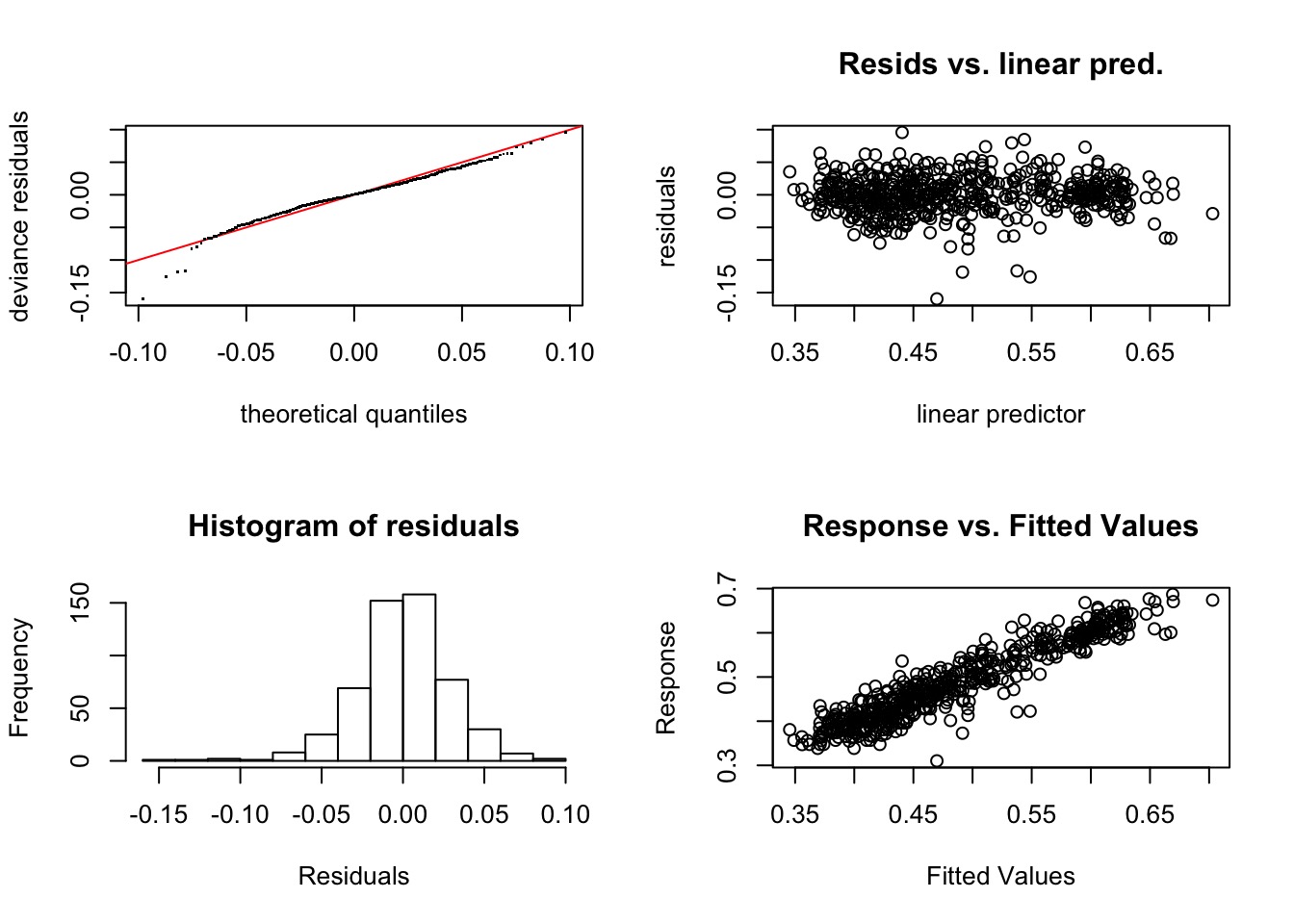
Method: GCV   Optimizer: magic
Smoothing parameter selection converged after 13 iterations.
The RMS GCV score gradient at convergence was 1.047426e-07 .
The Hessian was positive definite.
Model rank =  118 / 118 

Basis dimension (k) checking results. Low p-value (k-index<1) may
indicate that k is too low, especially if edf is close to k'.

          k'   edf k-index p-value
s(Wet)  9.00  2.73    1.00    0.49
s(T61)  9.00  2.45    0.98    0.26
s(x,y) 99.00 70.30    1.01    0.59

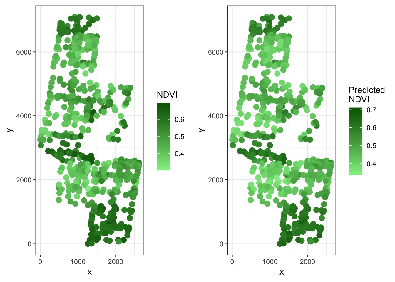
Compare Point Results to Observed Results

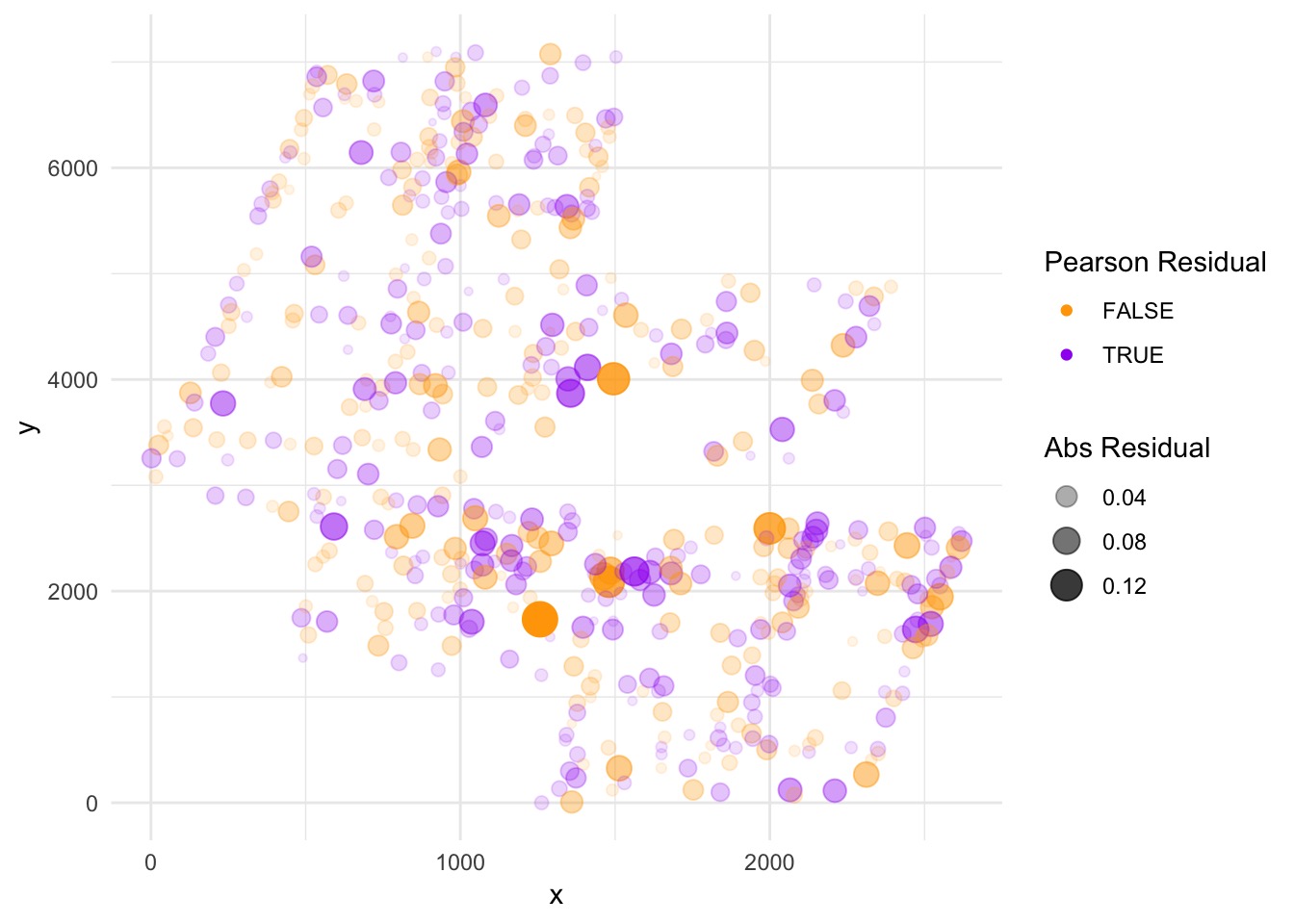
Residuals

Make this into a Map (Krig by Gam)

1. Come up with a spatial model of predictors
   
   
2. Make a grid of coordinates
   
   
3. Get krigged value of predictors at coordinates
   
   
4. Krig, baby, krig! With your gam.

Spatial Model of Predictors

fit.variogram(variogram(Wet ~ 1, 
              loc= ~x+y, data = boreal), 
              model = vgm(c("Gau", "Mat", "Sph")))

  model        psill    range
1   Nug 5.328932e-05    0.000
2   Sph 1.772570e-04 1461.766

fit.variogram(variogram(T61 ~ 1, 
              loc= ~x+y, data = boreal), 
              model = vgm(c("Gau", "Mat", "Sph")))

  model     psill    range kappa
1   Nug 0.0000000   0.0000   0.0
2   Mat 0.7272499 723.8632   0.5

Spatial Model of Predictors

#spherical
wet_mod <- gam(Wet ~ s(x,y, bs = "gp", m = 1, k=100), data = boreal)

#matern with low kappa
t_mod <- gam(T61 ~ s(x,y, bs = "gp", m = 3, k=100), data = boreal)

Make a Surface and Krig!

grid <- crossing(x = seq(min(boreal$x), max(boreal$x), length.out=100),
                 y = seq(min(boreal$y), max(boreal$y), length.out=100)
                 ) %>%
  
  #predictors
  mutate(Wet = predict(wet_mod, newdata = .),
         T61 = predict(t_mod, newdata = .)) %>%
  
  #response
  mutate(`Predicted NDVI` = predict(boreal_mod_spatial, newdata = .))

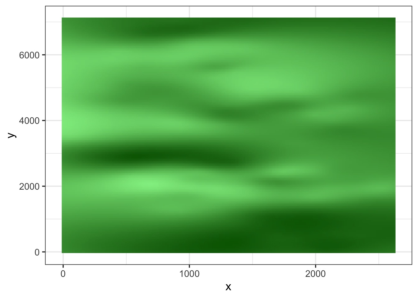
What’s it look like?

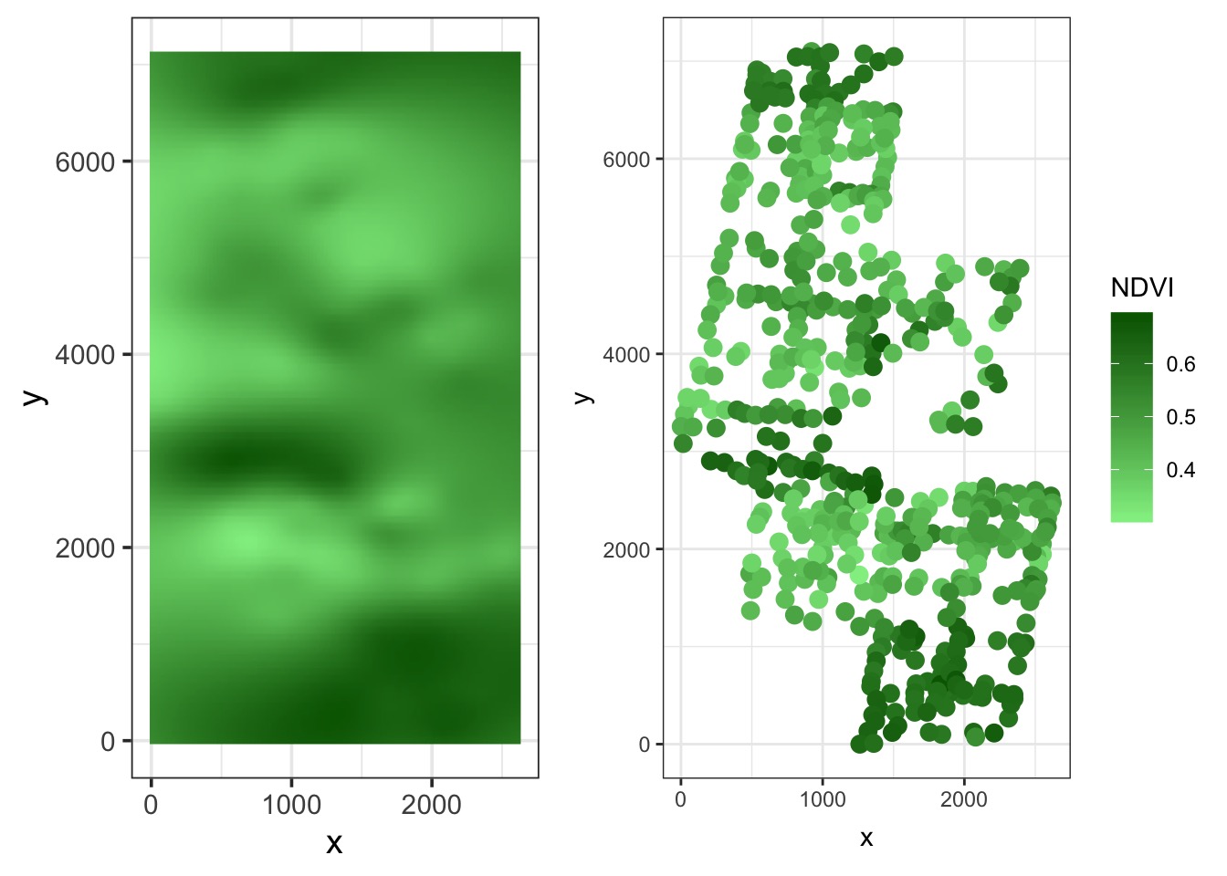
Compare to fit

What about Polygons?

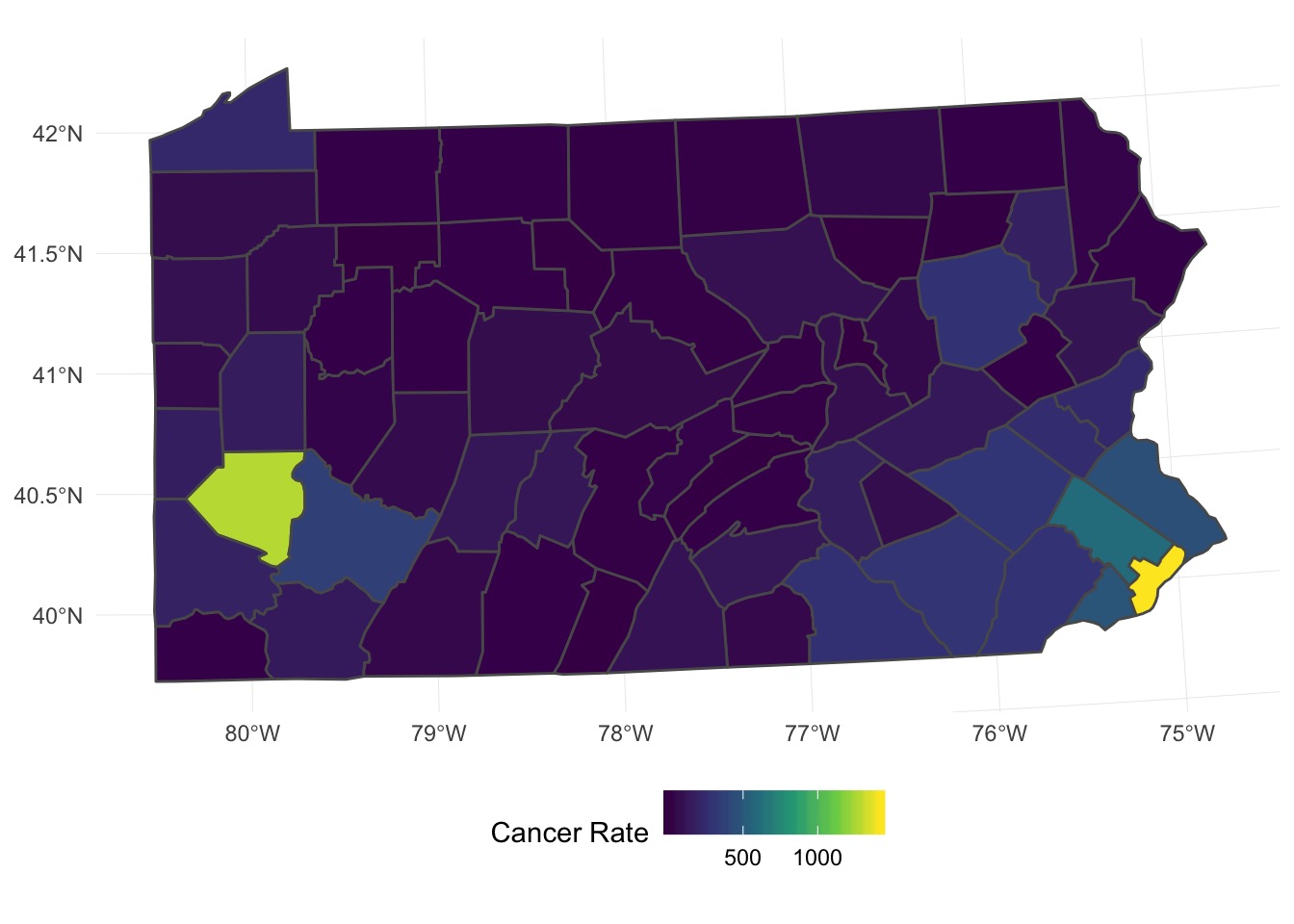
Many Things Underlying This Pattern

# A tibble: 1,071 x 7
   county cases population race  gender age          rate
   <fct>  <int>      <int> <fct> <fct>  <fct>       <dbl>
 1 adams      0       1492 o     f      Under.40 0       
 2 adams      0        365 o     f      40.59    0       
 3 adams      1         68 o     f      60.69    0.0147  
 4 adams      0         73 o     f      70+      0       
 5 adams      0      23351 w     f      Under.40 0       
 6 adams      5      12136 w     f      40.59    0.000412
 7 adams      5       3609 w     f      60.69    0.00139 
 8 adams     18       5411 w     f      70+      0.00333 
 9 adams      0       1697 o     m      Under.40 0       
10 adams      0        387 o     m      40.59    0       
# … with 1,061 more rows

We need a neighborhood matrix

We use the aggregated data, as there are 67 counties, not 1072!

library(spdep)

nb <- poly2nb(penn,  row.names = as.character(as.numeric(penn$county)))
names(nb) <- penn$county

Let’s Fit a Model!

# use 2 parallel threads, reduce if fewer physical CPU cores
ctrl <- gam.control(nthreads = 2) 


#The Binomial GAM
gam_mrf <- gam(cases/population ~ s(county, bs = 'mrf', 
                         xt = list(nb = nb)) +
                 race + gender + age, # define MRF smooth
               data = penn_sf,
               family = binomial(),
               weights = population) 

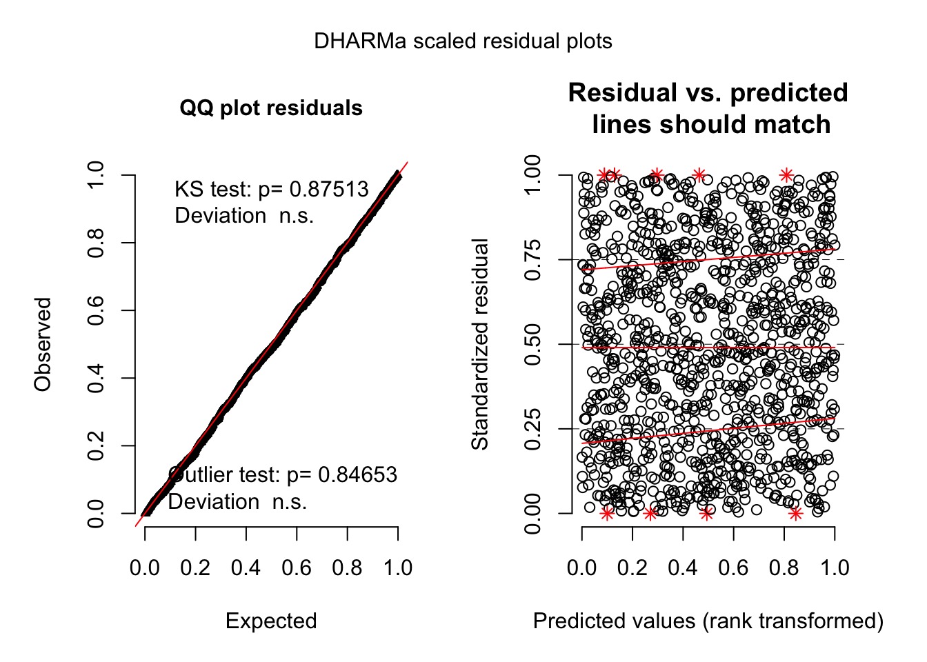
Did it work out?

library(DHARMa)
plot(simulateResiduals(gam_mrf))

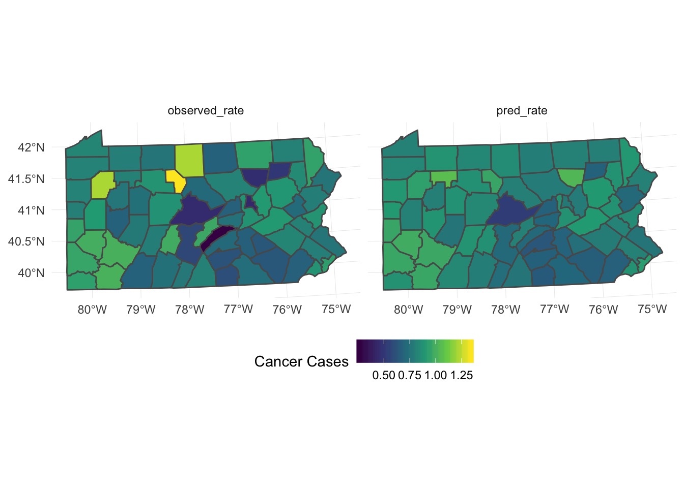
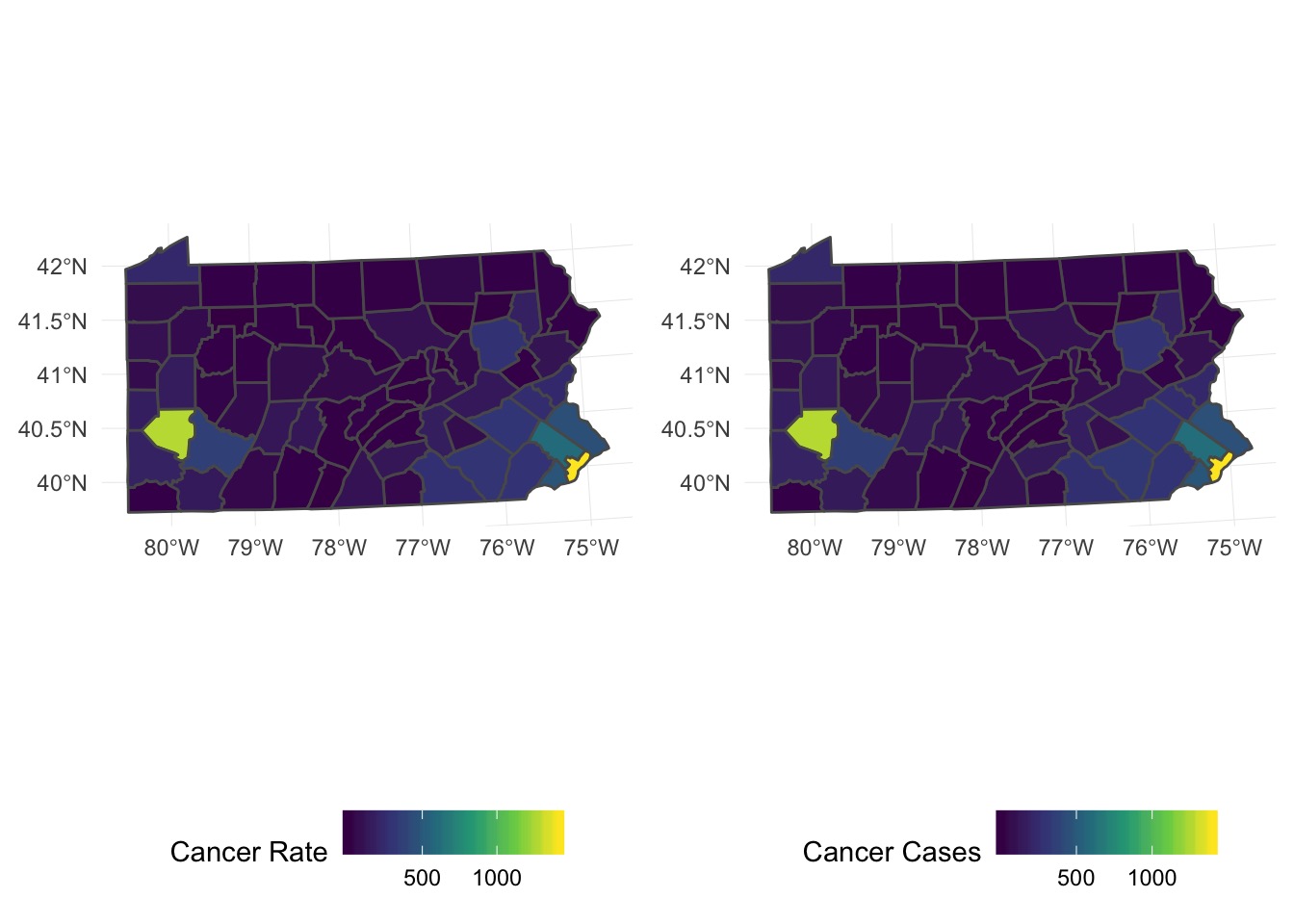
Do aggregated predictions match?

penn_sf <- penn_sf %>%
  mutate(pred_cases = fitted(gam_mrf)*population,
         pred_rate = fitted(gam_mrf))

#aggregate
penn_predict_agg <- penn_sf %>%
  group_by(county) %>%
  summarise(population = sum(population), 
            pred_cases = sum(pred_cases),
            pred_rate = sum(pred_cases)/population*1000,
            observed_rate = sum(cases)/population*1000) 

#plot side by side
pred_predict_plot <- ggplot(penn_predict_agg) +
  geom_sf(aes(fill = pred_cases)) +
  scale_fill_viridis_c(option = "D", guide = guide_colorbar("Cancer Cases")) +
  theme_minimal() + theme(legend.position="bottom")


penn_canc_poly + pred_predict_plot

Do aggregated predictions match?

What About Individual Predictions?

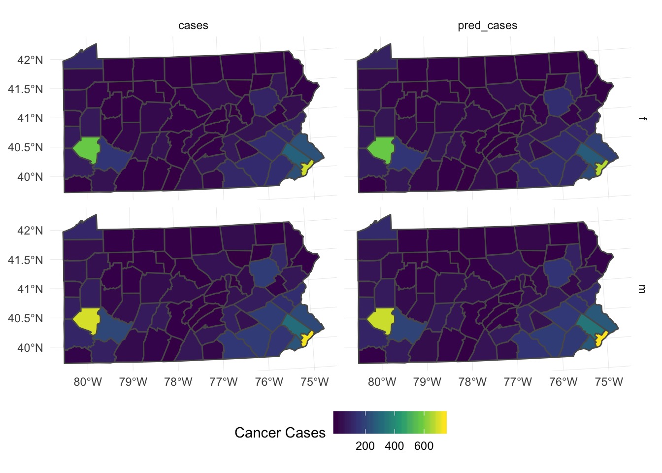
Comparing Rates

Looks like it’s underpredicting, although pattern is ok -