Spatial Autocorrelation with GLS

Much of our data is spatial

Much of our data is spatial

A note up front

• Spatial data analysis is… a big topic.
  
  
• Start by learning how to make maps (sf library)
  
  
• Be prepared to dive in. Deep.

To Space and Beyond

1. How do we assess spatial autocorrelation?

2. What are the possible patterns of spatial autocorrelation?

3. How do we assess point spatial data?

4. How do we assess polygon spatial data?

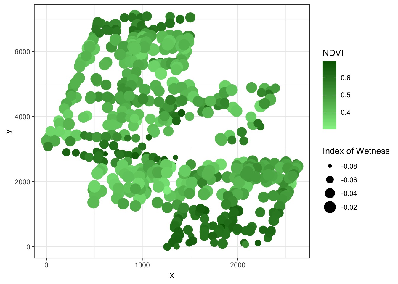
How correlated is NDVI across space?

Spatial Autocorrelation and Moran’s I

\[I = \frac{N}{W}\frac{\sum\sum w_{ij}(x_i - \bar{x})(x_j - \bar(x))}{\sum(x_i - \bar{x})^2}\]

• W is a weight matrix (1/pairwise distance) with diagonals of 0
  
• I = 1, perfect positive correlation, I = -1, perfect anti-correlation
  
• \(E_i = \frac{-1}{N-1}\) and can be tested

Calculating Moran’s I

1. Make a distance matrix

2. Convert it to a weight matrix

3. Run spdep::moran.test

Making a Weight Matrix

Yes, this is a PITA…

#first, mke a distance matrix of points
boreal_dists <- boreal %>%
  dplyr::select(x,y) %>% 
  dist() %>%
  as.matrix()

#inverse of distance is weight
boreal_dists_weights <- 1/boreal_dists
diag(boreal_dists_weights) <- 0

#turn into a weights list
boreal_w <- mat2listw(boreal_dists_weights)

• NB, use projections with true distances (e.g., UTM, not latlong)

Moran’s I

library(spdep)
moran.test(boreal$NDVI, boreal_w)

    Moran I test under randomisation

data:  boreal$NDVI  
weights: boreal_w    

Moran I statistic standard deviate = 45.157, p-value < 2.2e-16
alternative hypothesis: greater
sample estimates:
Moran I statistic       Expectation          Variance 
     1.834024e-01     -1.879699e-03      1.683501e-05 

What does this look like?

library(ncf)
boreal_cor <- spline.correlog(x=boreal$x, y=boreal$y,
                         z=boreal$NDVI, resamp=100, quiet=TRUE)

plot(boreal_cor)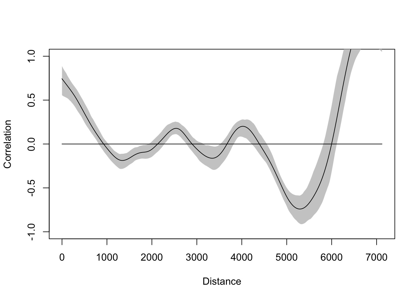

To Space and Beyond

1. How do we assess spatial autocorrelation?

2. What are the possible patterns of spatial autocorrelation?

3. How do we assess point spatial data?

4. How do we assess polygon spatial data?

SAR versus CAR

SAR:
Simultaneous Autoregressive Process \(y_i = BX_i + \sum Sy_ij + \epsilon_{i}\)

CAR:
Conditional Autoregressive Process \(y_i | y_{-i} ~\sim \mathcalc{N}{ BX_i + \sum S_{ij}yj, m_{ij}\)

SAR versus CAR

from https://stats.stackexchange.com/a/9983

Non-spatial model
My House Value is a function of my home Gardening Investment.

SAR model
My House Value is a function of the House Values of my neighbours.

CAR model
My House Value is a function of the Gardening Investment of my neighbours.

Variograms

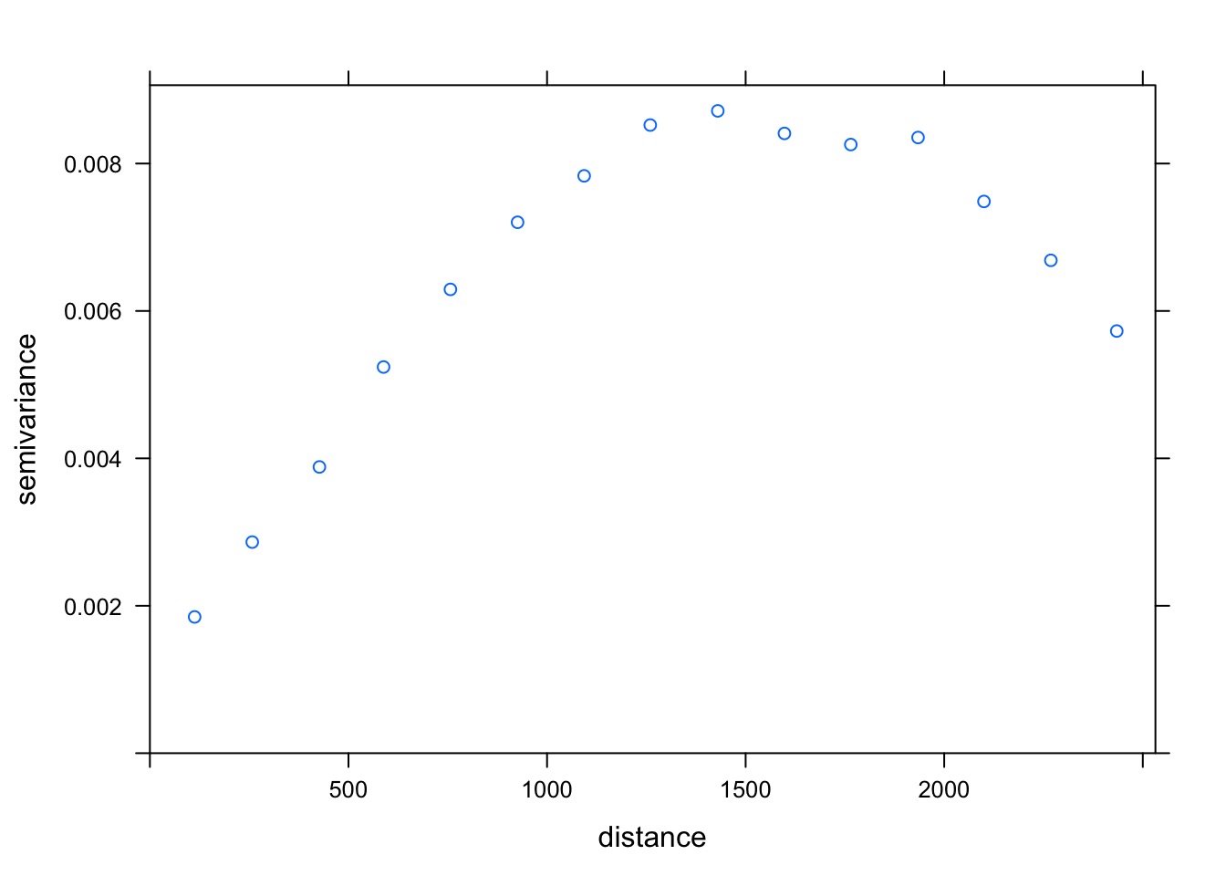
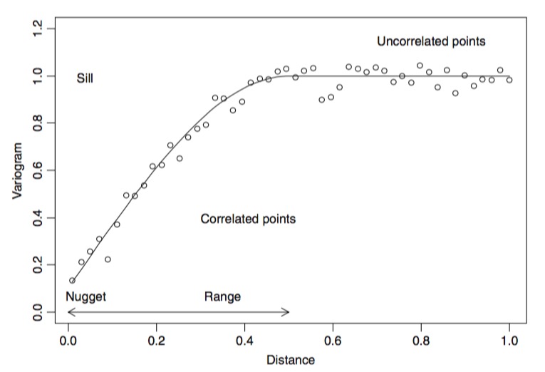
• (Semi)variograms allow us to look at variance of squared difference between points at different distances
  
  
• Computationally intensive
  
  
• Shape tells us what the correlation structure should be
  
  
• With a fit covariance function, can estimate the whole surface

Our Variogram

library(gstat)

v_boreal <- variogram(NDVI ~ 1, loc= ~x+y, data = boreal)
plot(v_boreal)

Anatomy of a Variogram

Spatial Correlation Matrix

\[ cor(\epsilon) = \begin{pmatrix} 1 & \rho_{ij} &\rho_{ik} & ... \\ \rho_{ji} & 1& \rho_jk & ...\\ \rho_{ki} & \rho_{kj} & 1 & ... \\ . & . & . & ... \\ . & . & . & ... \\ . & . & . & ... \\ \end{pmatrix}\]

\[\rho{ij} = f(x_i, x_j)\] e.g., \[\rho{ij} = exp(-Distance/range)\]

Different Shapes of Autocorrelation

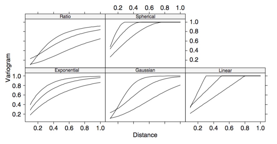
How do you tell the difference?

1. Biology
   
   
2. Fit all structures and evaluate
   
   
3. Visual examination of variogram shape

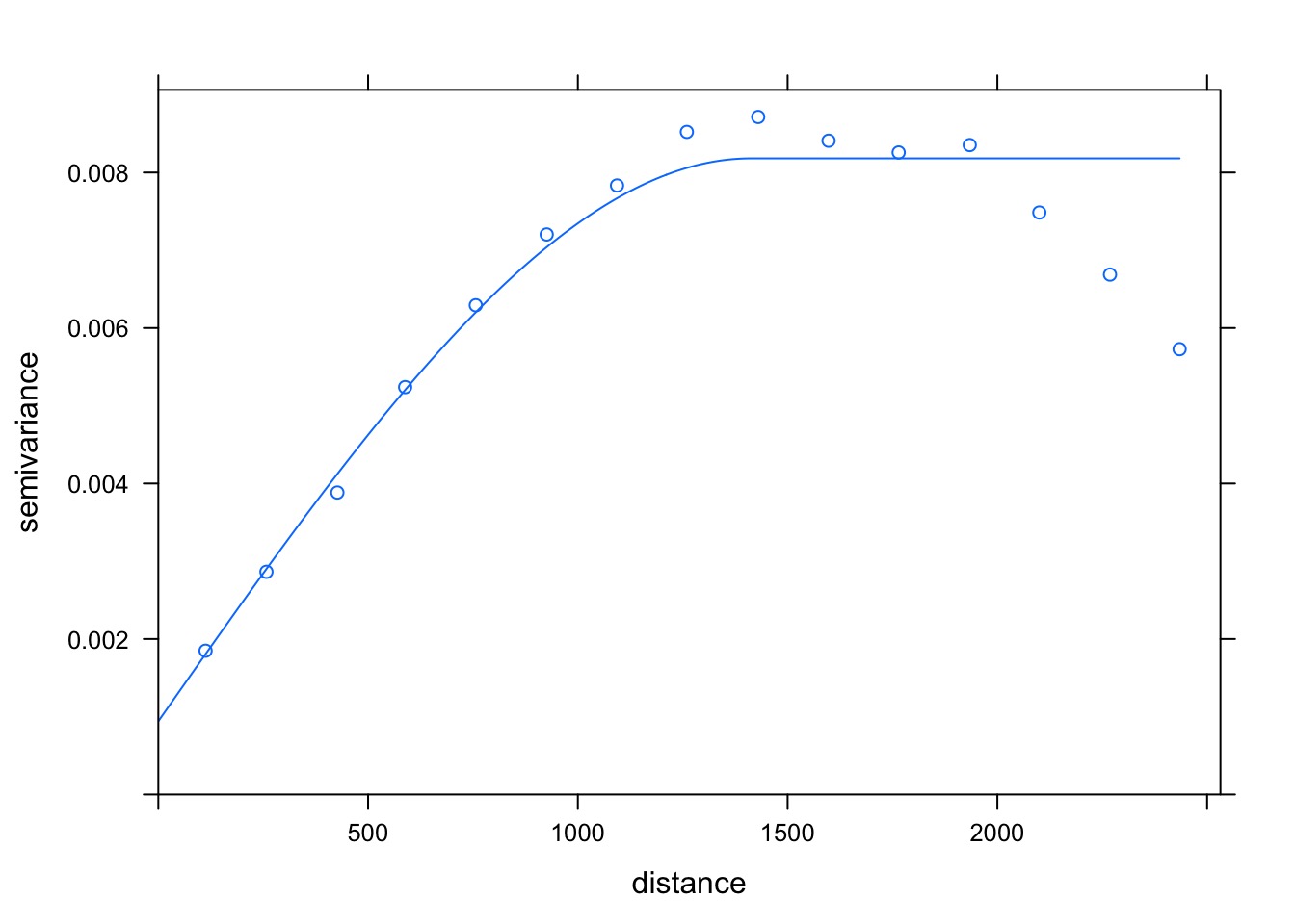
What model best describes our variogram?

best_vario <- fit.variogram(v_boreal, 
              model = vgm(c("Exp", "Gau", "Mat", "Sph")))

best_vario

  model        psill    range
1   Nug 0.0009415914    0.000
2   Sph 0.0072401874 1412.745

See the Fit Variogram

plot(v_boreal, model = best_vario)

What are the Implications of our Variogram: Krigging

1. Determine a model of the data (variogram!)
   
   
2. Build a grid covering the space you are interested in
   
   
3. Use your model to predict points between those you have measured

What are the Implications of our Variogram: Krigging

#1. Make a gstat object (model)
boreal_gstat <- gstat(formula = NDVI ~ 1, loc= ~x+y, 
                      data = boreal, model = best_vario)

#2. Create a grid of "Pixels" using x as columns and y as rows
TheGrid <- expand.grid(x=seq(1,3000, 100),y=seq(1,7000, 100))
coordinates(TheGrid)<- ~ x+y
#coordinates(boreal)<- ~ x+y
gridded(TheGrid) <- TRUE

#3. Make a predicted surface
TheSurface <- predict(boreal_gstat, model=best_vario, newdata=TheGrid)

#plot
image(TheSurface, col=terrain.colors(20),
      xlim = c(1,3e3), ylim = c(1, 7e3))

What are the Implications of our Variogram: Krigging

[using ordinary kriging]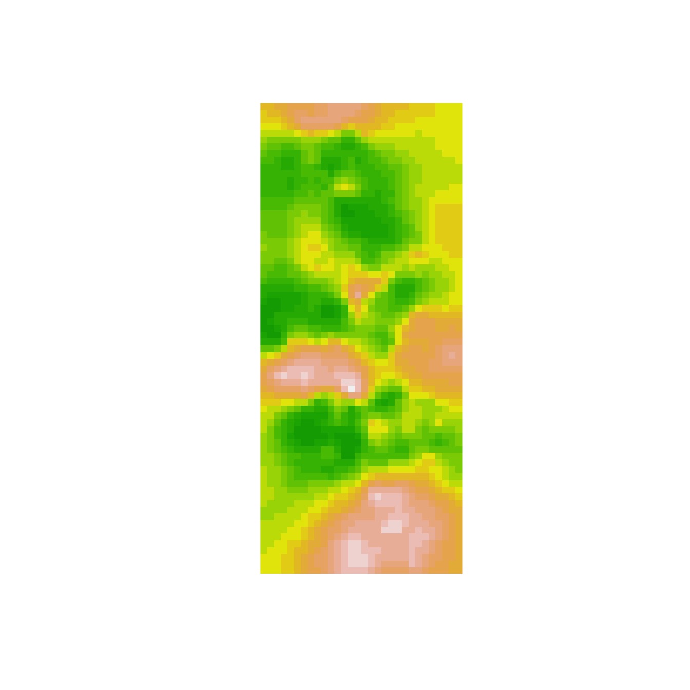

This is all very cool, but…

None of this involves biological processes

Model of Where Space Enters In

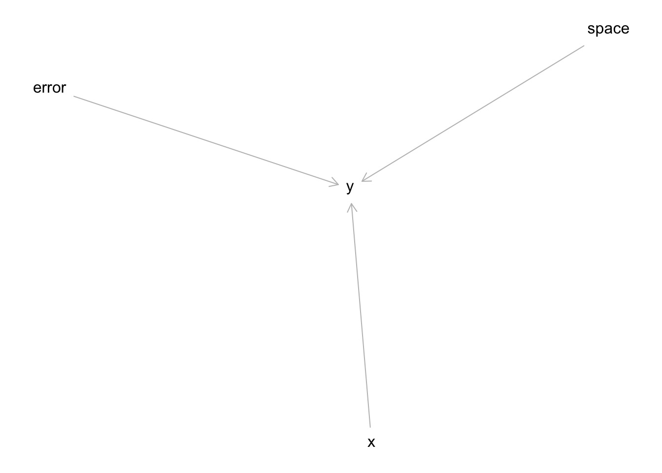
How do we translate this to correlation?

And…

Once we build a process-based understanding, we can krig even better!

To Space and Beyond

1. How do we assess spatial autocorrelation?

2. What are the possible patterns of spatial autocorrelation?

3. How do we assess point spatial data?

4. How do we assess polygon spatial data?

To Space and Beyond

1. How do we assess spatial autocorrelation?

2. What are the possible patterns of spatial autocorrelation?

3. How do we assess point spatial data?

4. How do we assess polygon spatial data?

Analysis of Point Pattern Data

Naieve Analysis of Point Pattern Data

boreal_mod <- lm(NDVI ~ Wet, data = as.data.frame(boreal))

Plot of Residuals

ggplot(boreal %>% mutate(resid = residuals(boreal_mod)),
       aes(x = x, y = y, color = resid)) +
  geom_point() + 
  scale_color_viridis_c(option = "B")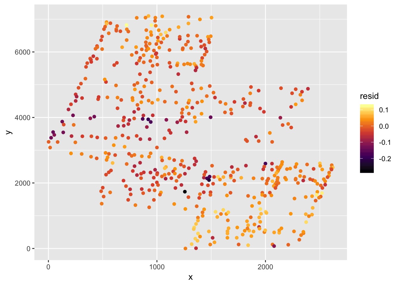

Analysis of Residuals

moran.test(residuals(boreal_mod), boreal_w)

    Moran I test under randomisation

data:  residuals(boreal_mod)  
weights: boreal_w    

Moran I statistic standard deviate = 30.255, p-value < 2.2e-16
alternative hypothesis: greater
sample estimates:
Moran I statistic       Expectation          Variance 
     1.217804e-01     -1.879699e-03      1.670611e-05 

What’s the Variogram of Residuals?

v_bor_resid <- variogram(residuals(boreal_mod) ~ 1, loc= ~x+y, data = boreal)
plot(v_bor_resid)

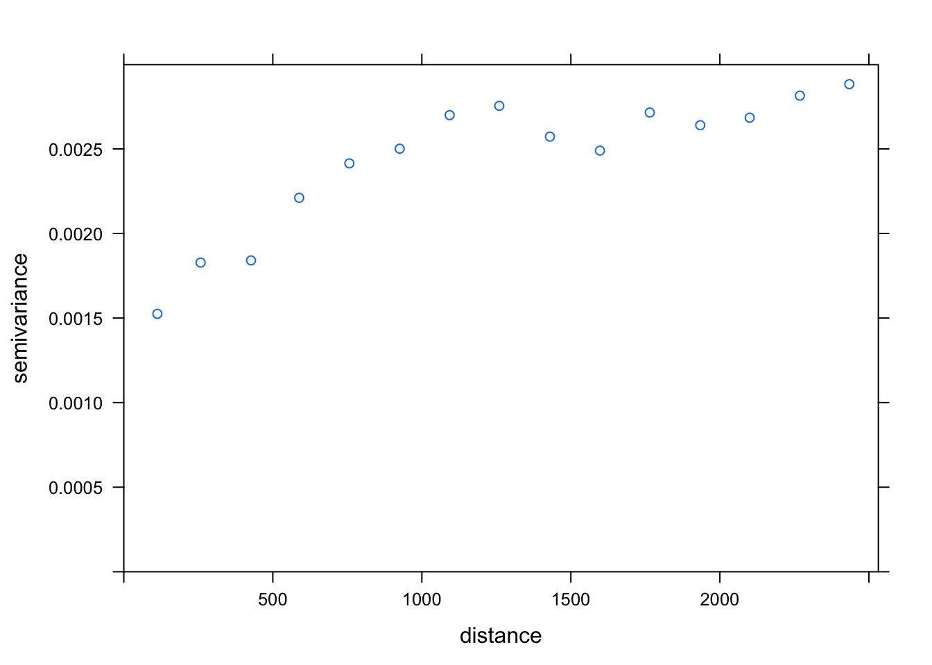
What model best describes our residuals?

best_resid_vario <- fit.variogram(v_bor_resid, 
              model = vgm(c("Exp", "Gau", "Mat", "Sph")))

best_vario

  model        psill    range
1   Nug 0.0009415914    0.000
2   Sph 0.0072401874 1412.745

Compensating with CAR Model

library(brms)
bor_brms  <- brm(NDVI ~ Wet,
                 family = gaussian(),
                 autocor = cor_car(W = boreal_dists),
                 data = boreal)

Compensating with CAR Model: glmmTMB

library(glmmTMB)

#get things prepped
boreal <- boreal %>% 
  mutate(position = numFactor(x, y),
         group = factor(1))

bor_tmb  <- glmmTMB(NDVI ~ Wet + exp(position + 0 | group),
                 family = gaussian(),
                 data = boreal)

Compensating with CAR Model: gls

library(nlme)

bor_gls  <- gls(NDVI ~ Wet,
                correlation = corSpher(form = ~ x+y),
                 data = boreal)

Differences?

library(broom.mixed)

tidy(boreal_mod)

# A tibble: 2 x 5
  term        estimate std.error statistic   p.value
  <chr>          <dbl>     <dbl>     <dbl>     <dbl>
1 (Intercept)    0.327   0.00552      59.3 1.95e-236
2 Wet           -4.88    0.154       -31.6 3.05e-124

tidy(bor_gls)

# A tibble: 2 x 5
  term        estimate std.error statistic  p.value
  <chr>          <dbl>     <dbl>     <dbl>    <dbl>
1 (Intercept)    0.402     9.19     0.0437 9.65e- 1
2 Wet           -3.04      0.168  -18.1    1.62e-57

Predictions Across Landscape

1. Requires predictions of wetness across landscape
   
   
2. So, variogram and krig away!
   
   
3. Then make a new grid.
   
   
4. Use wetness values and spatial values to simulate new landscape with predict and brms or glmmTMB model

To Space and Beyond

1. How do we assess spatial autocorrelation?

2. What are the possible patterns of spatial autocorrelation?

3. How do we assess point spatial data?

4. How do we assess polygon spatial data?

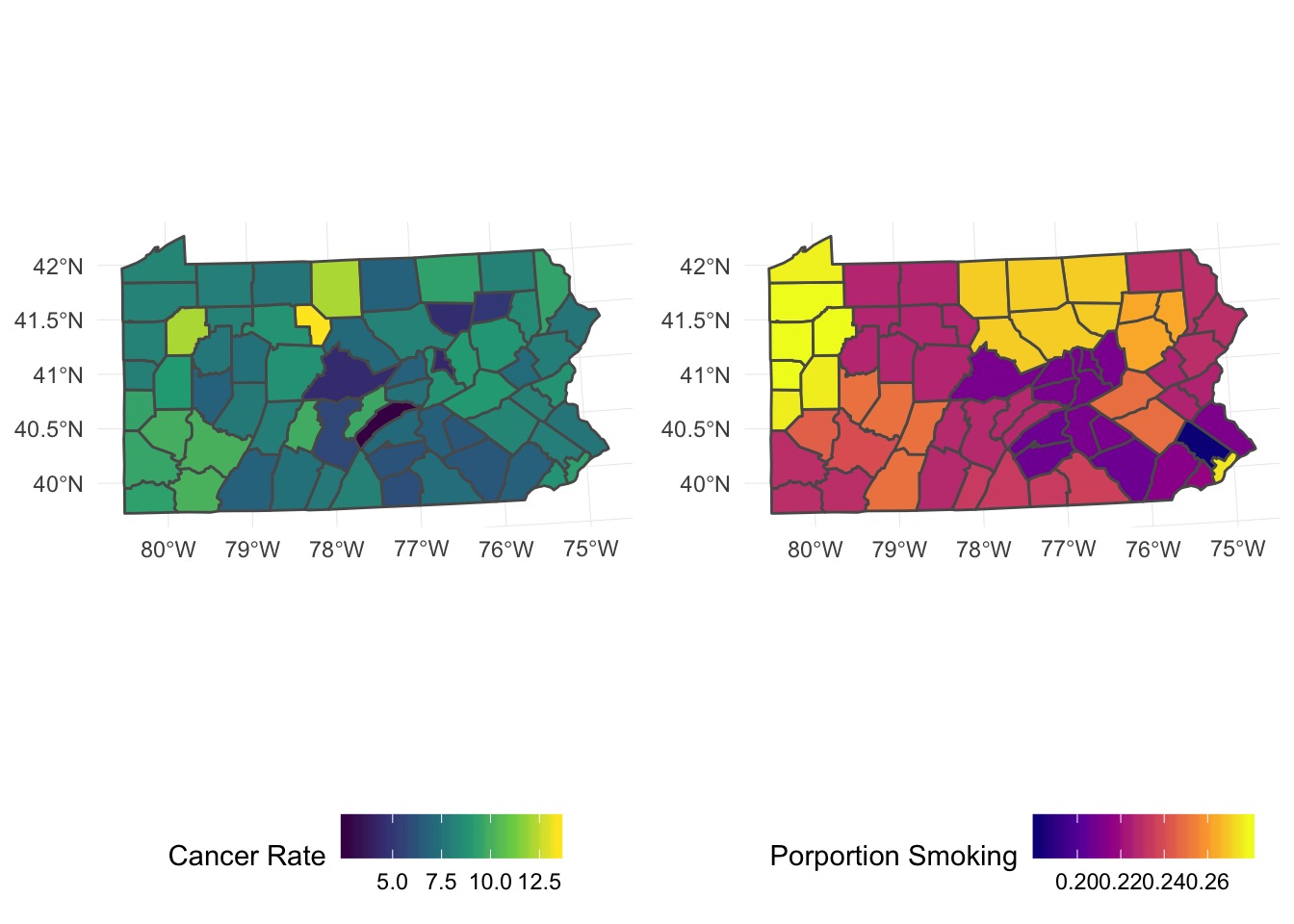
Analysis of Polygons

We need distances - So let’s Make a Mesh

penn_mesh <- poly2nb(penn)
coords <- st_centroid(st_geometry(penn))

plot(penn_mesh, coords, col = "red")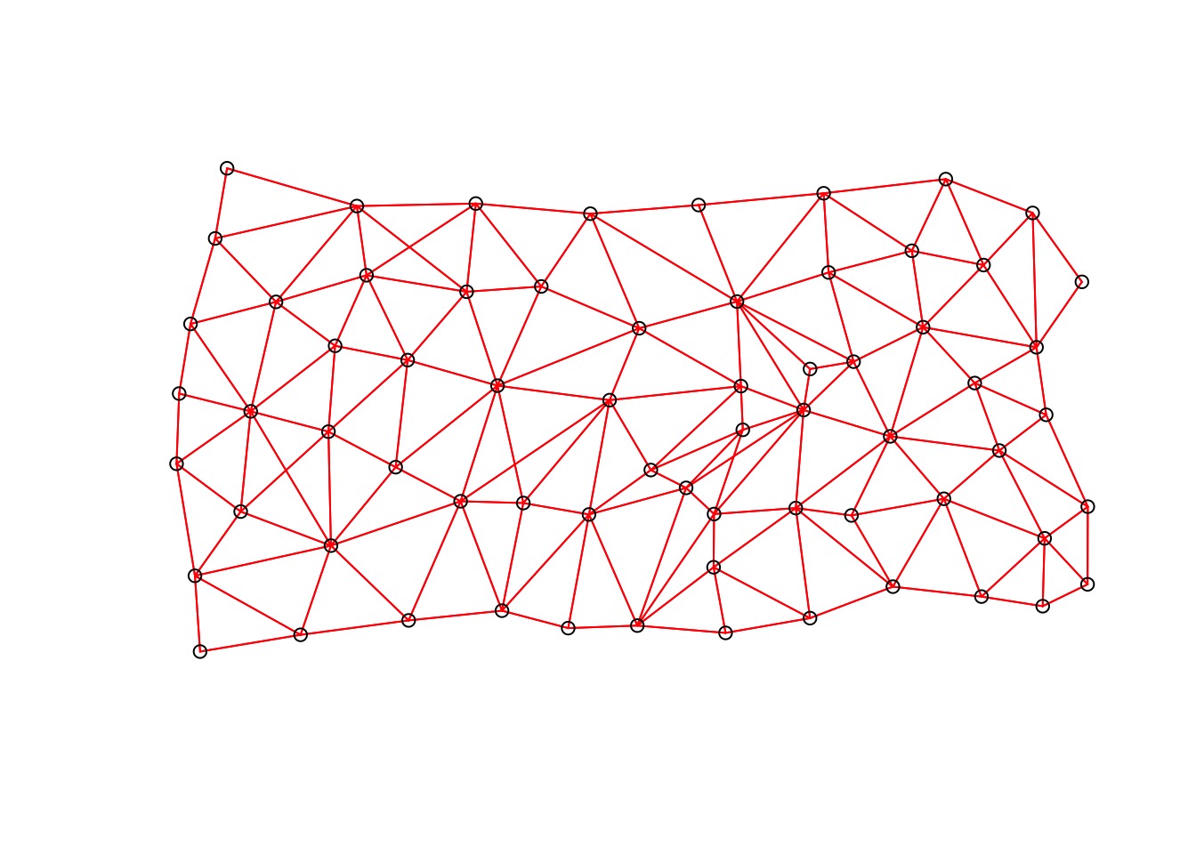

Analysis of Autocorrelation Says….

    Moran I test under randomisation

data:  residuals(penn_mod)  
weights: penn_weights    

Moran I statistic standard deviate = 0.60877, p-value = 0.2713
alternative hypothesis: greater
sample estimates:
Moran I statistic       Expectation          Variance 
      0.030083778      -0.015151515       0.005521394 

Really?

penn_v <- variogram(residuals(penn_mod) ~ 1, 
          ~x+y, 
          data = as.data.frame(penn) %>%
            mutate(x = st_coordinates(coords)[,1],
                   y = st_coordinates(coords)[,2]))

plot(penn_v)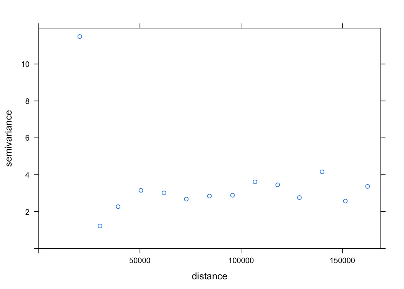

Fitting A SAR Model Anyway…

library(spatialreg)

penn_sar <- spautolm(rate ~ smoking, 
                     data = penn,
                     listw = penn_weights)

compare

             Estimate Std. Error  t value   Pr(>|t|)
(Intercept)  3.621208   2.135931 1.695377 0.09478954
smoking     18.345216   8.944603 2.050982 0.04430385

             Estimate Std. Error  z value   Pr(>|z|)
(Intercept)  3.715435   2.161831 1.718652 0.08567779
smoking     17.919386   9.048019 1.980476 0.04765004

Predictions?

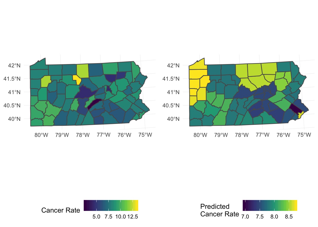
Example

1. Irish forest data
   
   
2. Goal is to model lake Ph
   
   
3. Possible influences:
   • Sodium Dominance Index (SDI)
     
   • Status as forested or not
   • Altitude
     
     
4. Spatial autocorrelation possible