Interaction Effects

What is an interaction effect?
- Effects of predictors no longer independent
- Effects conditional on one another
- Effects conditional on one another
- May not be possible to evluate effect of single predictor in isolation
- Generalized linear models: All predictors interact (even with themselves)
- Effect of a variable dependent on current value of all other predictors
- Effect of a variable dependent on current value of all other predictors
- Multilevel models: slope/intercept vary by groups
- interactions all the way down
Linear nteractions with Discrete Variables
- Variable slope
- Contrast to just plain olde variable intercept
- Contrast to just plain olde variable intercept
- Effect of a predictor (even intercept!) depends on what group it’s in
- Gateway to multilevel/mixed models
How does ruggedness influence GDP?
data(rugged)
rugged$log_gdp <- log(rugged$rgdppc_2000)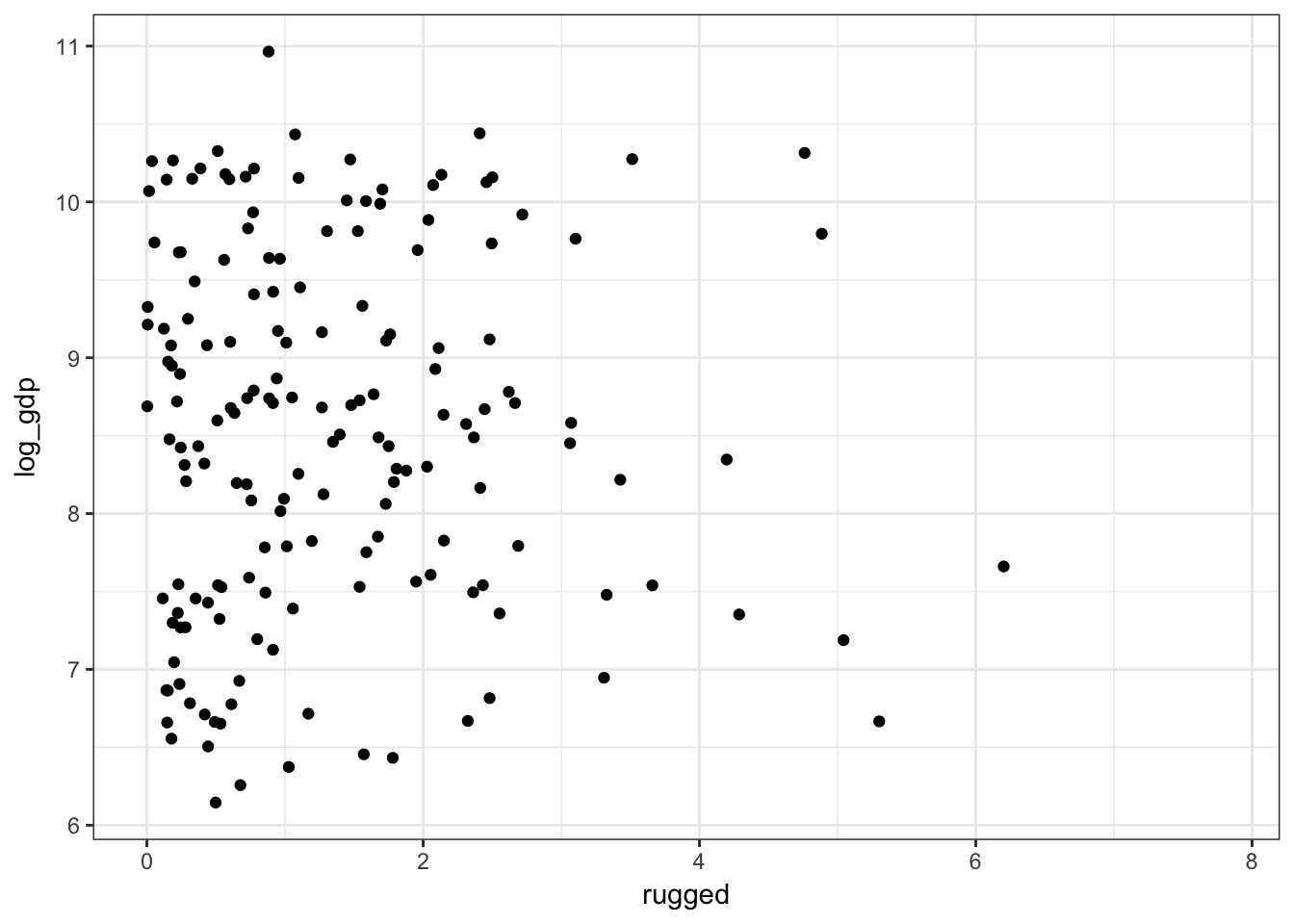
How does ruggedness influence GDP?
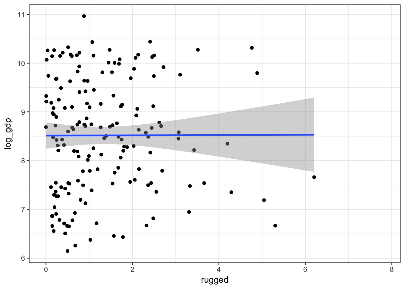
How does ruggedness influence GDP?
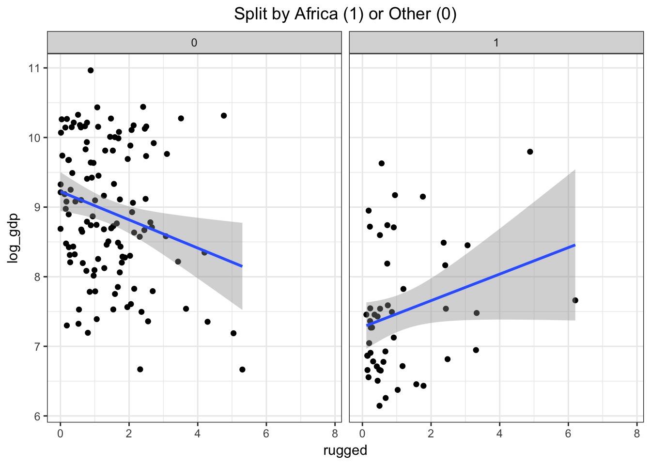
Model with No Interaction
#prep the data
d <- rugged[complete.cases(rugged$log_gdp),]

#need indices >0
d$cont_africa <- d$cont_africa +1

#The model
mod_no_int <- alist(
  #likelihood
  log_gdp ~ dnorm(mu, sigma),

  #data generating process
  mu <- bA[cont_africa] + bR*rugged,

  #priors
  bR ~ dnorm(0,1),
  bA[cont_africa] ~ dnorm(8,100),
  sigma ~ dunif(0,10))

fit_no_int <- map(mod_no_int, data=d)
What does that look like?
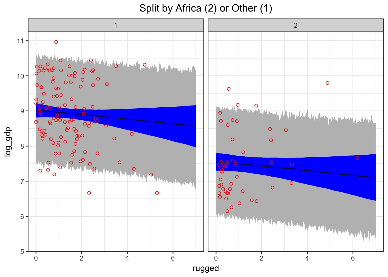
Handling Categories
No Interaction:
mu <- bA[cont_africa] + bR*rugged,

#OR

mu <- a + bA[cont_africa] + bR*rugged,OK, so, How do we write a categorical interaction?
Interaction 1:
mu <- bA[cont_africa] + bR*rugged,

bR <- bR_0 + bR_1*cont_africa- Keeps form for
mubut incorporates new information
bR_1is difference from non-African bR
OK, so, How do we write a categorical interaction?
Interaction 2
mu <- bA[cont_africa] + bR*rugged + bR_1*cont_africa,- More compact
bR_1has same meaning as before
OK, so, How do we write a categorical interaction?
Interaction 3
mu <- bA[cont_africa] + bR[cont_africa]*rugged,- Uses indexing for groups
- No post-hoc calculation issues
The full model
int_mod <- alist(
  #likelihood
  log_gdp ~ dnorm(mu, sigma),

  #Data generating process
  mu <- bR[cont_africa]*rugged + bA[cont_africa],

  #priors - note indexing!
  bR[cont_africa] ~ dnorm(0,1),
  bA[cont_africa] ~ dnorm(8,100),
  sigma ~ dunif(0,10)
)

int_fit <- map(int_mod, data=d)
Coefficients
Note depth=2 for groups
precis(int_fit, depth=2, cor=TRUE) Mean StdDev 5.5% 94.5% bR___1 bR___2 bA___1 bA___2 sigma
bR[1] -0.20 0.08 -0.32 -0.08 1.00 0.00 -0.79 0.00 0
bR[2] 0.19 0.10 0.02 0.36 0.00 1.00 0.00 -0.66 0
bA[1] 9.22 0.14 9.00 9.44 -0.79 0.00 1.00 0.00 0
bA[2] 7.28 0.18 6.99 7.56 0.00 -0.66 0.00 1.00 0
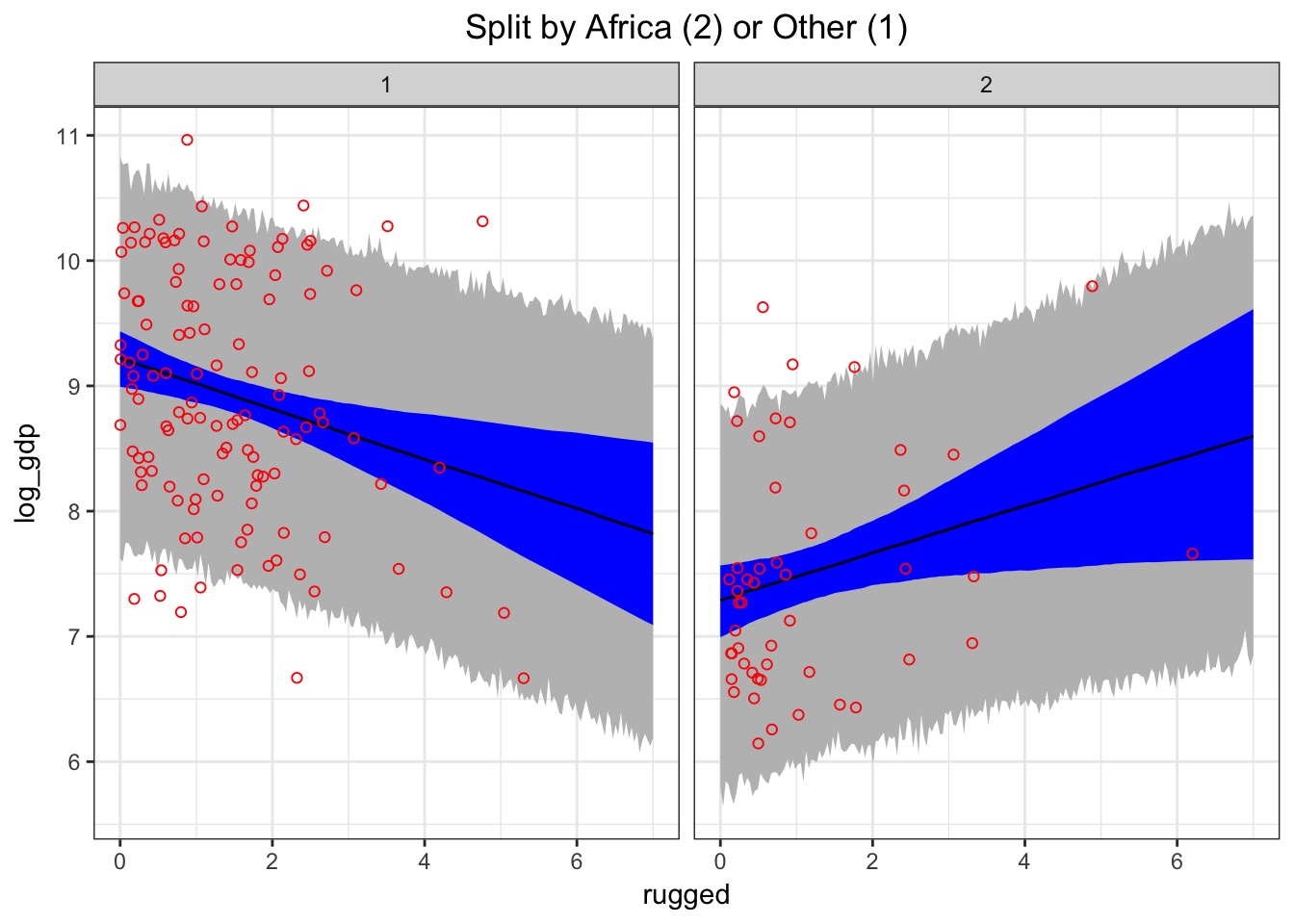
sigma 0.93 0.05 0.85 1.01 0.00 0.00 0.00 0.00 1bR changes in sign between groups!
Inspection
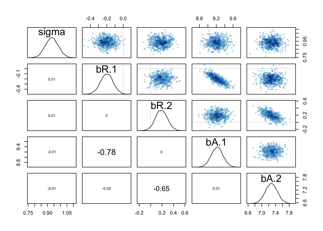
A posthoc: Are slopes really different?
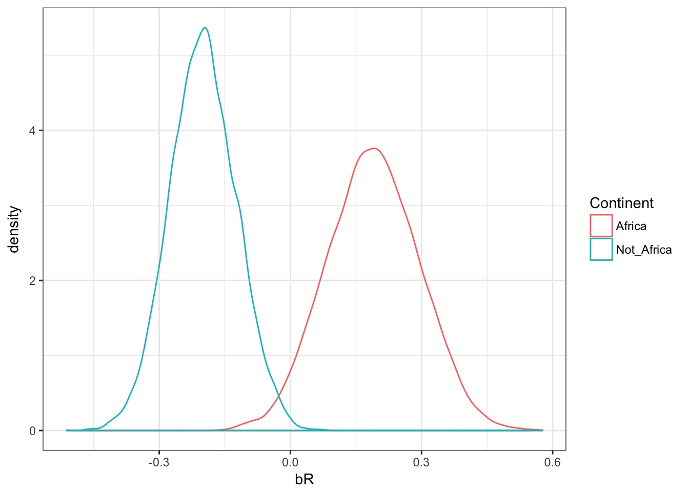
Calculate the difference
samps <- extract.samples(int_fit)

names(samps)
[1] "sigma" "bR" "bA" head(samps$bR) [,1] [,2]
[1,] -0.15179570 0.27818267
[2,] -0.17523714 0.09972111
[3,] -0.15245867 0.34652585
[4,] -0.09268935 0.11231884
[5,] -0.14039837 0.25779016
[6,] -0.19623546 0.21929095#Not Africa v. Africa
diff_br <- samps$bR[,1] - samps$bR[,2]Were they different?
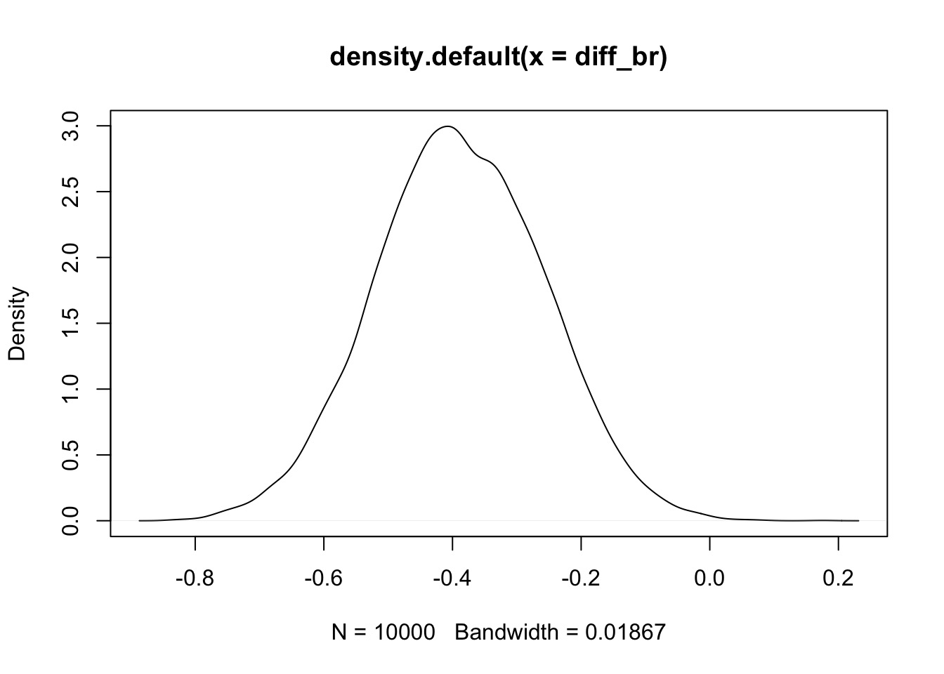
99.9% were < 0
They are quite likely different
Interpretation
What can you say so far?
Continuous Interactions
- Effects of predictors no longer independent
- Effects conditional on one another
- Effects conditional on one another
- May not be possible to evluate effect of single predictor in isolation
- Require counterfactual plots to assess meaning
Tulips!

data(tulips)
head(tulips)
bed water shade blooms
1 a 1 1 0.00
2 a 1 2 0.00
3 a 1 3 111.04
4 a 2 1 183.47
5 a 2 2 59.16
6 a 2 3 76.75Continuous Interactions are Simple to Code
tulip_mod <- alist(
  #likelihood
  blooms ~ dnorm(mu, sigma),

  #Data generating process
  mu <- a + bW*water + bS*shade + bWS*water*shade,

  #priors
  a ~ dnorm(130,100),
  bW ~ dnorm(0,100),
  bS ~ dnorm(0,100),
  bWS ~ dnorm(0,100),
  sigma ~ dunif(0,100)
)
Common fitting errors!
fit_tulip <- map(tulip_mod, data=tulips)Error in map(tulip_mod, data = tulips): non-finite finite-difference value [5]
Start values for parameters may be too far from MAP.
Try better priors or use explicit start values.
If you sampled random start values, just trying again may work.
Start values used in this attempt:
a = 150.331309039261
bW = 187.446212728008
bS = -41.3825724654428
bWS = 80.3598233487261
sigma = 60.5601385002956Fixes
- Try a different algorithm
Nelder-Meadoften works, but slower
SANNalso works, but sloooow
- Transform values
- Center
- Scale
- Supply start values
- Change priors
- Change algorithmic parameters
These both work
fit_tulip_1 <- map(tulip_mod,
                   data=tulips,
                   method="Nelder-Mead")
or
tulip_cent <- tulips %>% mutate(shade = shade-mean(shade),
                                          water = water-mean(water))
fit_tulip_2 <- map(tulip_mod,
                   data=tulip_cent)
How does the meaning change with centering?
      fit_tulip_1 fit_tulip_2
a      -49.50      128.98
bW     136.79       74.97
bS      20.49      -41.12
bWS    -33.70      -51.95
sigma   47.37       45.25
nobs       27          27
And, what do these coefficients say?
Counterfactal Plots are Necessary
tulip_pred_df <- crossing(shade = -1:1, water = -1:1)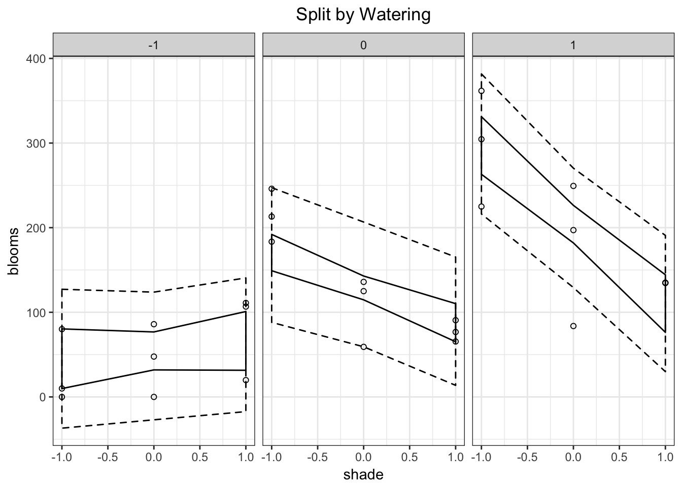
Exercise
- Take the excellent milk models you have!
- Now, make models where
- Effects vary by clade AND/OR
- Different predictors interact
- Effects vary by clade AND/OR
- Evaluate with WAIC
- Plot implications to understand
- Single model or ensemble
- Single model or ensemble
- Go green if you have something cool to throw up