Information Theory and a Multimodel World

How complex a model do you need to be useful?

Some models are simple but good enough

More Complex Models are Not Always Better or Right

Consider this data…

sppnames <- c( "afarensis","africanus",
               "habilis","boisei",
               "rudolfensis","ergaster","sapiens")

brainvolcc <- c( 438 , 452 , 612, 521, 752, 871, 1350 )
masskg <- c( 37.0 , 35.5 , 34.5 , 41.5 , 55.5 , 61.0 , 53.5 )

d <- data.frame( species=sppnames, 
                 brain=brainvolcc, 
                 mass=masskg )

Underfitting

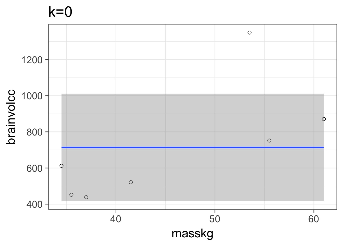
We have explained nothing!

Overfitting

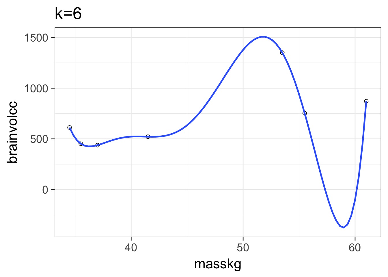
We have perfectly explained this sample

What is the right fit?

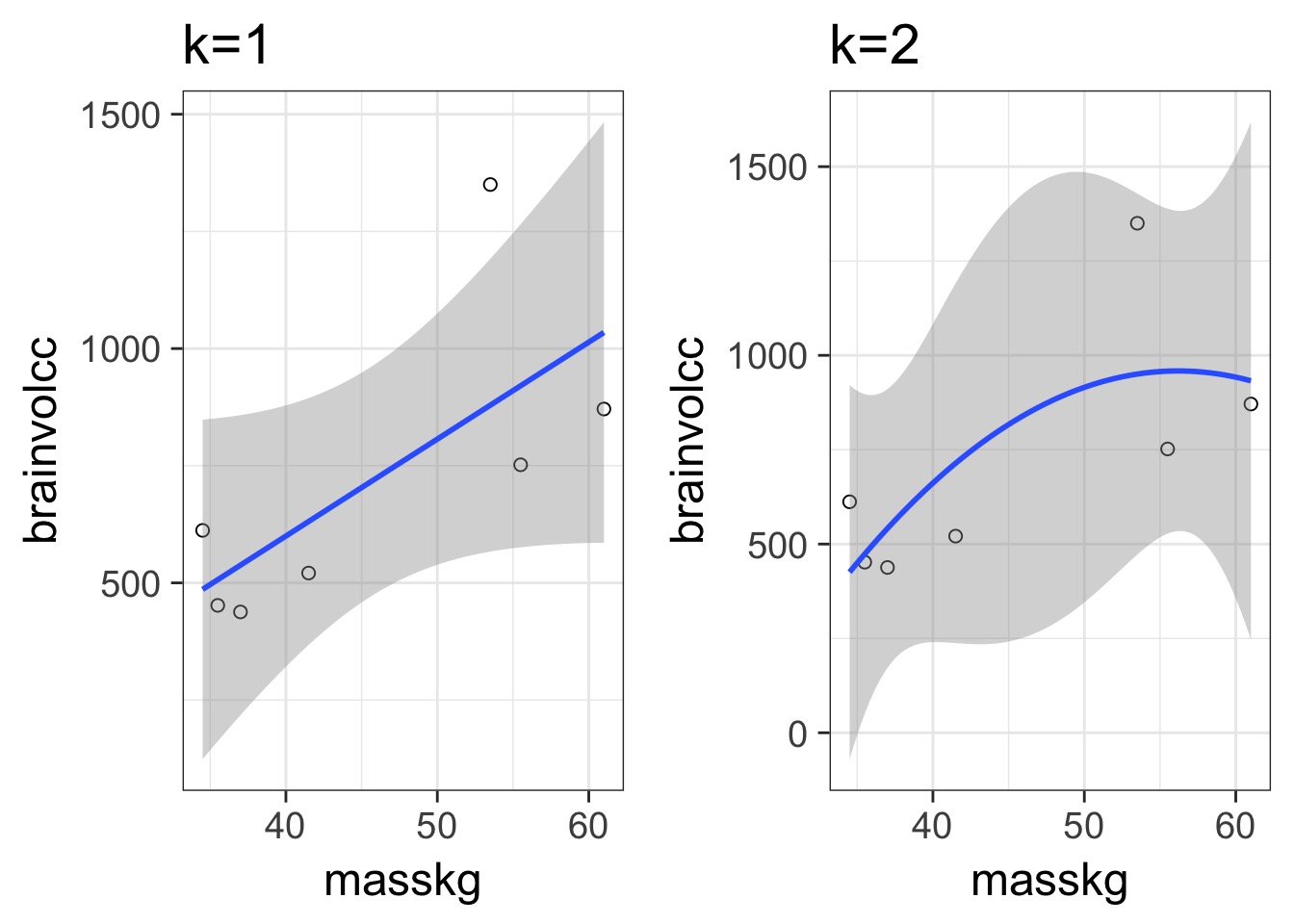
How do we Navigate?

Regularization
- Penalize parameters with weak support
Optimization for Prediction
- Information Theory
- Draws from comparison of information loss

In and Out of Sample Deviance

Deviance = -2 * log(dnorm(\(y_i | \mu_i\)))

The deviance of this linear regression is 3.176628510^{5}

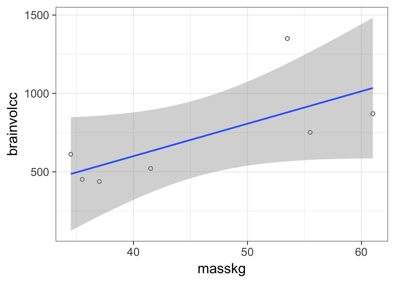
In and Out of Sample Deviance

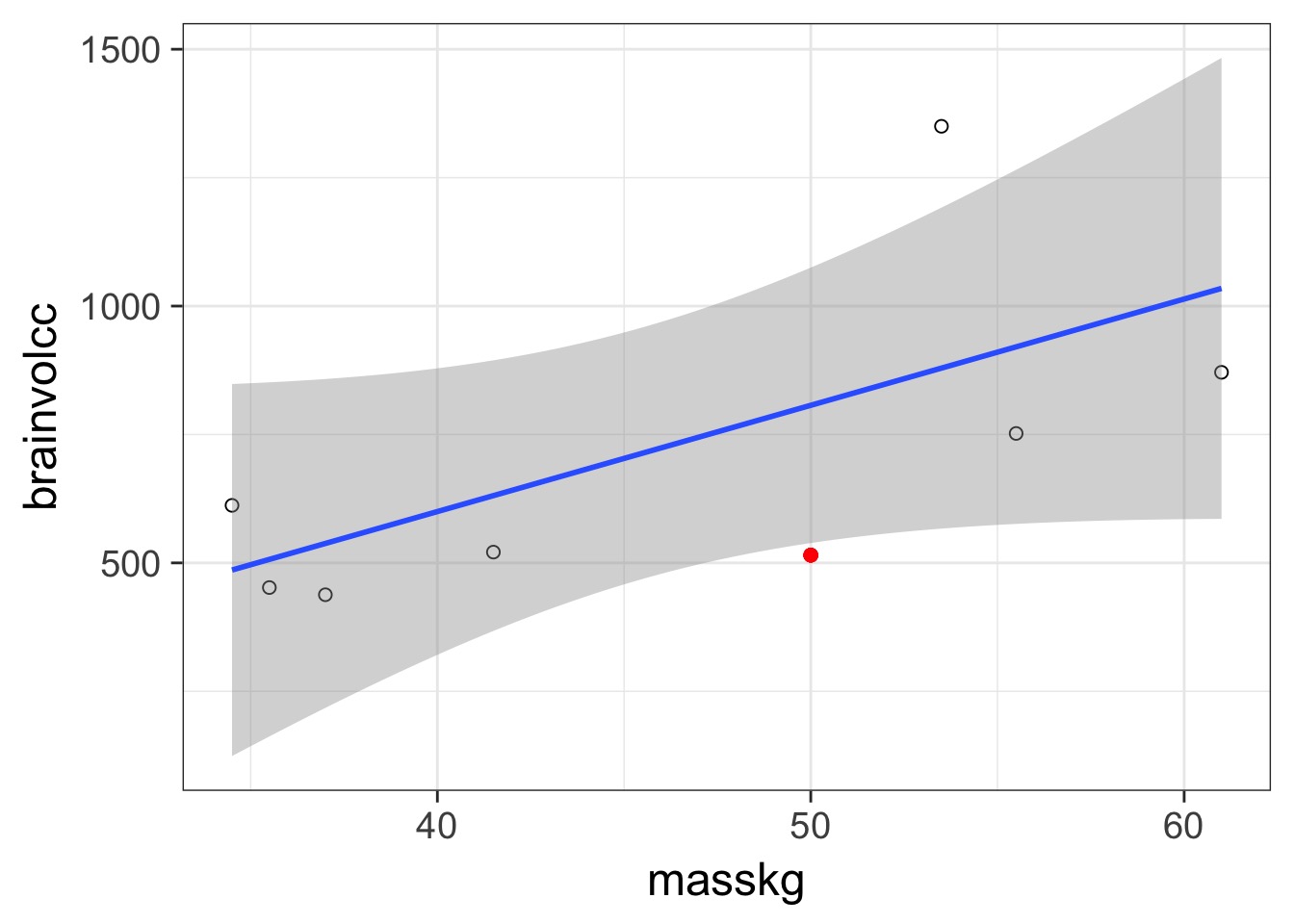
Prediction: 806.8141456, Observe: 515
Deviance: 8.526583810^{4}

In and Out of Sample Deviance

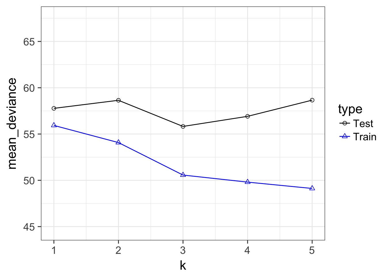
Our Goal for Judging Models

Can we minimize the out of sample deviance
So, fit a model, and evaluate how different the deviance is for a training versus test data set is
What can we use to minimize the difference?

Regularlization

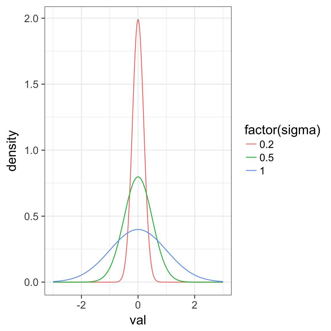
- Regularization means shrinking the prior towards 0

- Means data has to work harder to overcome prior

- Good way to shrink weak effects with little data, which are often spurious

- But, requires significant tuning

Regularization and Train-Test Deviance

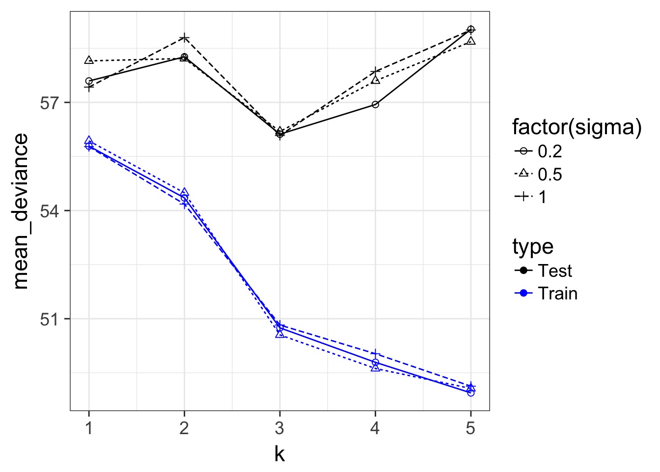
A Criteria Estimating Test Sample Deviance

What if we could estimate out of sample deviance?
The difference between training and testing deviance shows overfitting

A Criteria Estimating Test Sample Deviance

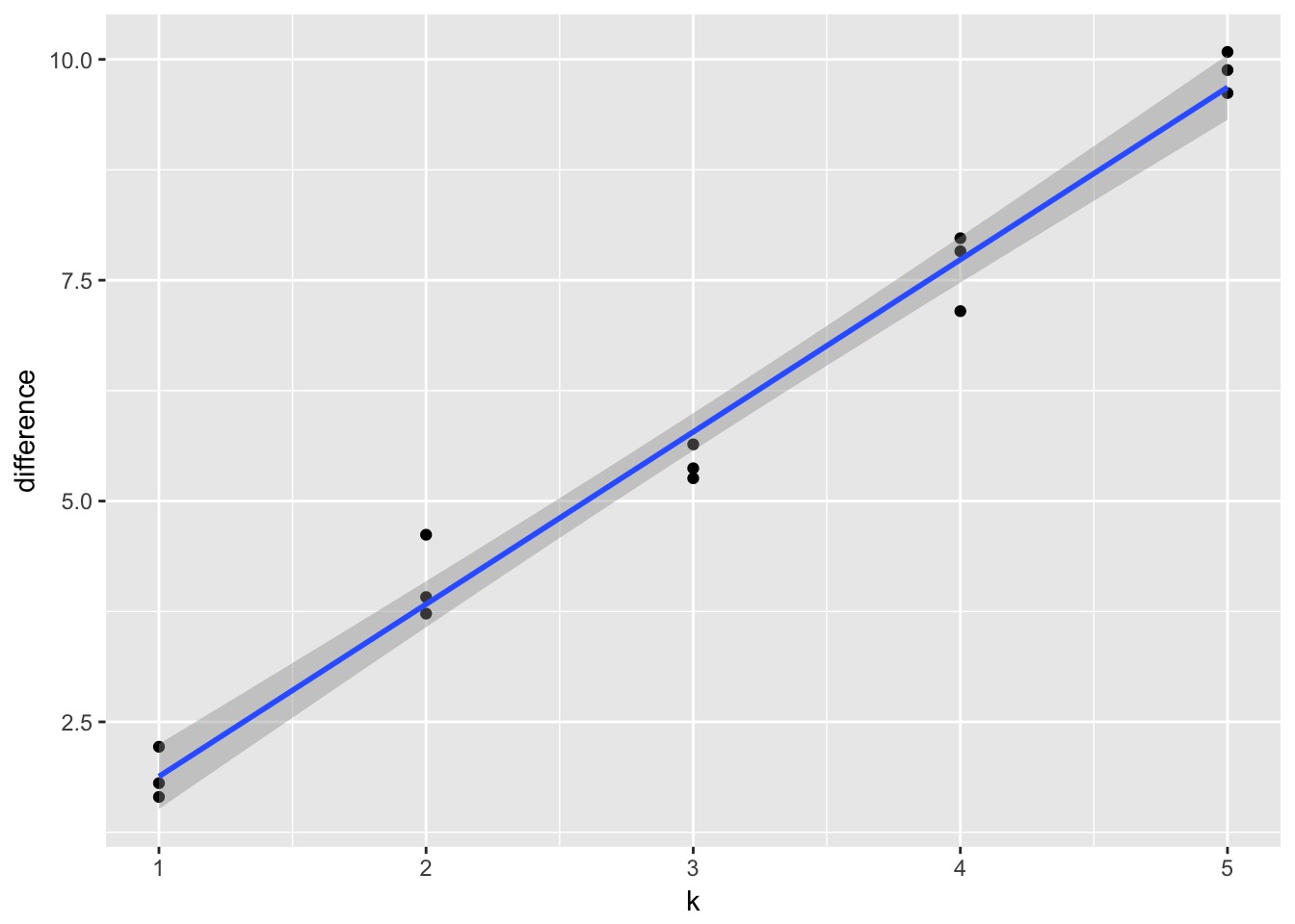Slope here of 1.95

AIC

So, \(E[D_{test}] = D_{train} + 2K\)
This is Akaike’s Information Criteria (AIC)

\[AIC = Deviance + 2K\]

AIC

AIC optimized for forecasting (out of sample deviance)
Requires flat priors
Assumes large N relative to K
- AICc for a correction
Difficult to define in a mixed model context

What about IC in Bayes?

We do estimate the posterior distribution of the deviance
Average of the posterior, \(\bar{D}\) is our \(D_{train}\)
But what about # of parameters?
- For a non-mixed model, this is not a concern - just the AIC
- For a mixed model…trickier

Effective number of Parameters

In addition to \(\bar{D}\), there is also \(\hat{D}\)
- The value of the posterior at the posterior mean
Given Bayesian logic:
- \(\bar{D}\) is our estimate of the out of sample deviance
- \(\hat{D}\) is our \(D_{train}\)
- So, \(\bar{D} - \hat{D}\) = number of parameters
We term this \(p_D\) for effective number of parameters

DIC

\[DIC = 2 \bar{D} - 2 p_D\]

DIC

\[DIC = 2 \bar{D} - 2 p_D\]

Works well for multivariate normal posteriors
Handles mixed models
Reduces to AIC with flat priors
But does not require flat priors - which does interesting things to \(p_D\)!
But… fails with anything non-normal, and hot debate on even mixed effects

And so we pause…

Our goal is to maximize prediction
Why not look at the pieces that make up the deviance
- The pointwise predictive power of the posterior
We can define the Pr(y_i | posterior simulations)
This tells us the distribution of the predictive power of our posterior for each point
\(llpd = \sum log Pr(y_i | \theta)\)

But what about Parameters?

We know that as k increases, our uncertainty in coefficients increases
As uncertainty increases, Pr(y_i | simulations) widens
Thus, this variance gives us an effective penalty term
\(p_{waic} = \sum Var(log Pr(y_i | \theta))\)

Widely Applicable IC

\[WAIC = -2 \sum log Pr(y_i | \theta) + 2 \sum Var(log Pr(y_i | \theta))\]

\[= -2 llpd + 2 p_{waic}\]

Wantanabe’s Information Criteria

Advantage in being pointwise is that we also get an estimate of uncertainty

Disadvantage that inaprporpiate to use with lagged (spatial or temporal) predictors

Which should I use?

AIC for flat priors, fixed effects is fine
Adding priors, mixed models, DIC or WAIC
Non-gaussian posterior? WAIC
Lagged predictors? DIC

How do I use my IC?

We can calculate:

\[w_{i} = \frac{e^{\Delta_{i}/2 }}{\displaystyle \sum^R_{r=1} e^{\Delta_{i}/2 }}\]
Where \(w_{i}\) is the relative support for model i making the best prediction compared to other models in the set being considered.

Model weights summed together = 1

Monkies and Milk

data(milk)
d <- milk[ complete.cases(milk) , ]
d$neocortex <- d$neocortex.perc / 100

A lotta Models

a.start <- mean(d$kcal.per.g)
sigma.start <- log(sd(d$kcal.per.g))

#null
m6.11 <- map(
    alist(
        kcal.per.g ~ dnorm( a , exp(log.sigma) )
    ) ,
    data=d , start=list(a=a.start,log.sigma=sigma.start) )

#neocortex only
m6.12 <- map(
    alist(
        kcal.per.g ~ dnorm( mu , exp(log.sigma) ) ,
        mu <- a + bn*neocortex
    ) ,
    data=d , start=list(a=a.start,bn=0,log.sigma=sigma.start) )

A lotta Models

# log(mass) only
m6.13 <- map(
    alist(
        kcal.per.g ~ dnorm( mu , exp(log.sigma) ) ,
        mu <- a + bm*log(mass)
    ) ,
    data=d , start=list(a=a.start,bm=0,log.sigma=sigma.start) )

# neocortex + log(mass)
m6.14 <- map(
    alist(
        kcal.per.g ~ dnorm( mu , exp(log.sigma) ) ,
        mu <- a + bn*neocortex + bm*log(mass)
    ) ,
    data=d , start=list(a=a.start,bn=0,bm=0,log.sigma=sigma.start) )

A WAIC

WAIC( m6.14 )

[ 100 / 1000 ]
[ 200 / 1000 ]
[ 300 / 1000 ]
[ 400 / 1000 ]
[ 500 / 1000 ]
[ 600 / 1000 ]
[ 700 / 1000 ]
[ 800 / 1000 ]
[ 900 / 1000 ]
[ 1000 / 1000 ]

[1] -15.08076
attr(,"lppd")
[1] 12.33633
attr(,"pWAIC")
[1] 4.795952
attr(,"se")
[1] 7.68153

Comparing Models

milk.models <- compare( m6.11 , m6.12 , m6.13 , m6.14 )
milk.models

       WAIC pWAIC dWAIC weight   SE  dSE
m6.14 -14.5   5.1   0.0   0.91 7.61   NA
m6.13  -8.3   2.8   6.2   0.04 5.53 5.34
m6.11  -8.0   1.9   6.5   0.04 4.68 7.24
m6.12  -6.0   3.0   8.5   0.01 4.28 7.51

Comparing Models

plot(milk.models, cex=1.5)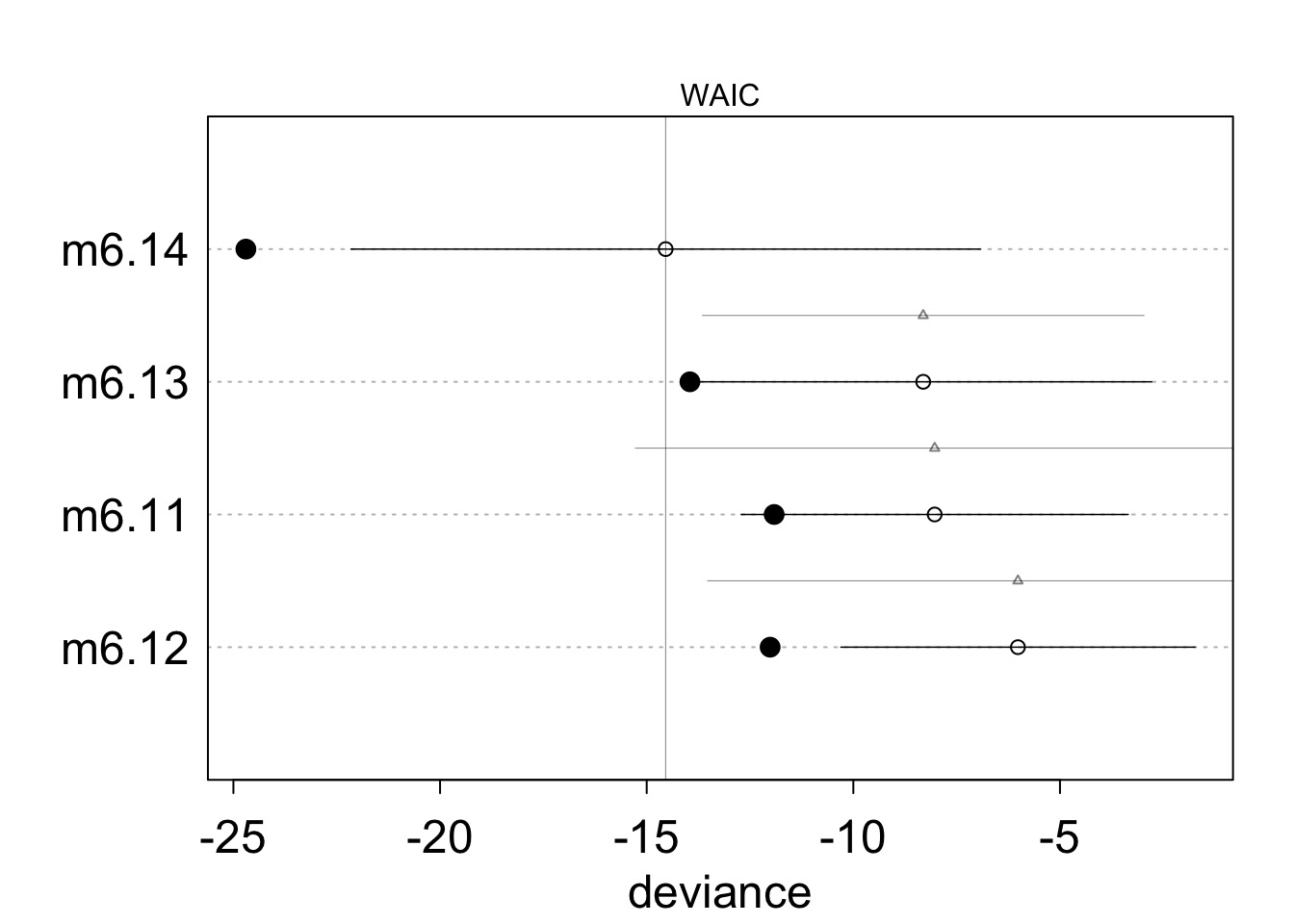

solid = deviance, circle=WAIC, triangle = \(\Delta\)WAIC

Death to model selection

While sometimes the model you should use is clear, more often it is not
Further, you made those models for a reason: you suspect those terms are important
Better to look at coefficients across models
For actual predictions, ensemble predictions provide real uncertainty

Coefficients

Remember, m6.14 has a 97% WAIC model weight

ctab <- coeftab( m6.11 , m6.12 , m6.13 , m6.14)
ctab

          m6.11   m6.12   m6.13   m6.14  
a            0.66    0.35    0.71   -1.09
log.sigma   -1.79   -1.80   -1.85   -2.16
bn             NA    0.45      NA    2.79
bm             NA      NA   -0.03   -0.10
nobs           17      17      17      17

Coefficients

Remember, m6.14 has a 97% WAIC model weight

plot(ctab)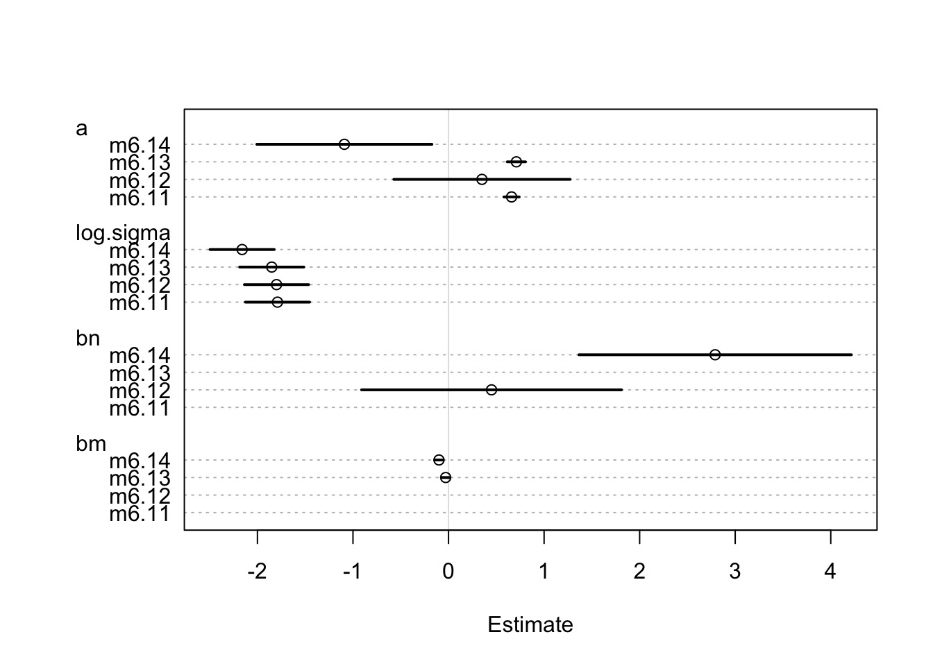

Ensemble Prediction

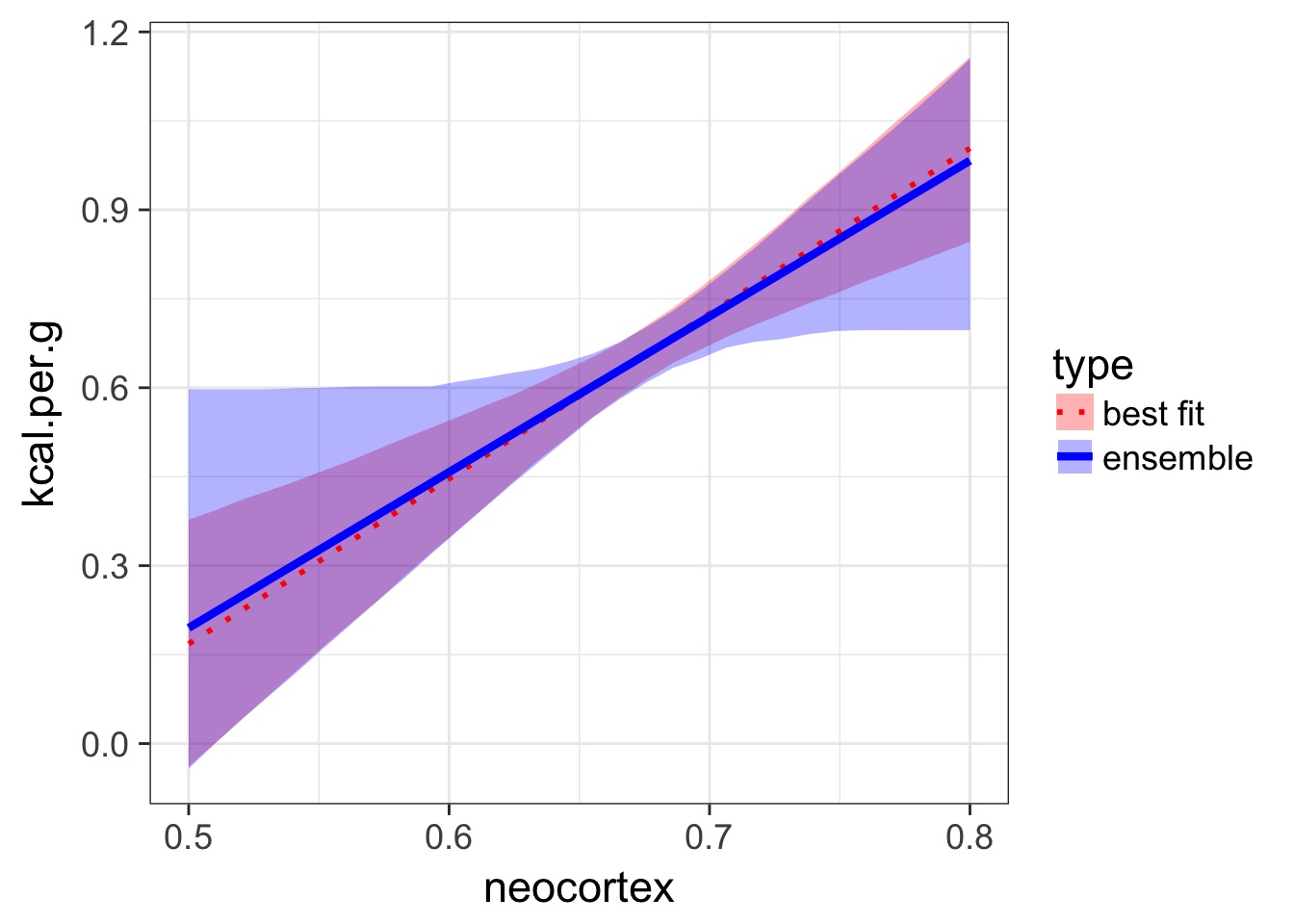
Ensemble prediction gives us better uncertainty estimates
Takes relative weights of predictions into account
Takes weights of coefficients into account
Basicaly, get simulated predicted values, multiply them by model weight

Making an Ensemble

milk.ensemble <- ensemble( m6.11, m6.12, 
                           m6.13 ,m6.14 , data=d.predict )

mu_ensemble <- apply( milk.ensemble$link , 2 , mean )
mu.PI_fit <- apply( milk.ensemble$link , 2 , PI )

Making an Ensemble

Exercise

Take your milk multiple predictor models with clade, milk components, both, and neither
Compare via WAIC
Get ensemble predictions for each clade