Bayesian Linear Regression

Why Linear Regression: A Simple Statistical Golem
- Describes association between predictor and response
- Response is additive combination of predictor(s)
- Constant variance
Why should we be wary of linear regression?
- Approximate
- Not mechanistic
- Often deployed without thought
- But, often very accurate
Why a Normal Error Distribution
- Good descriptor of sum of many small errors
- True for many different distributions
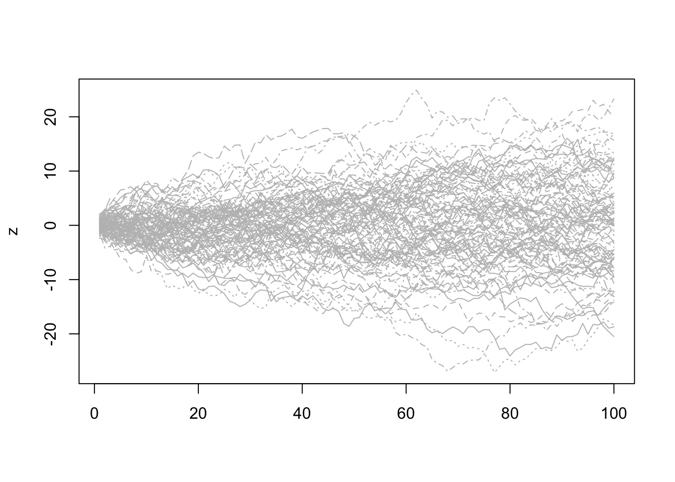
Why a Normal Error Distribution
Flexible to Many distributions
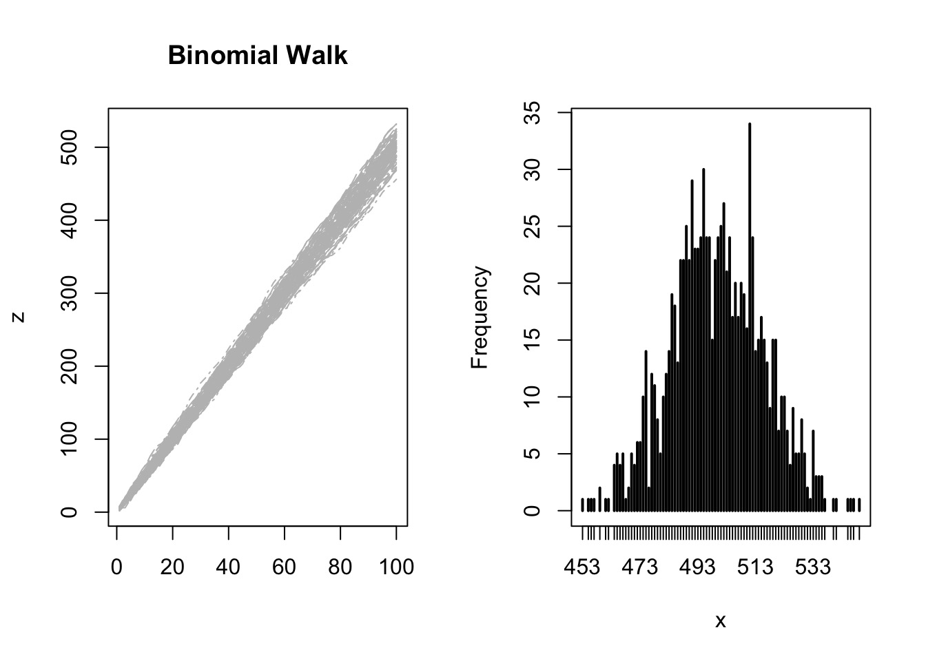
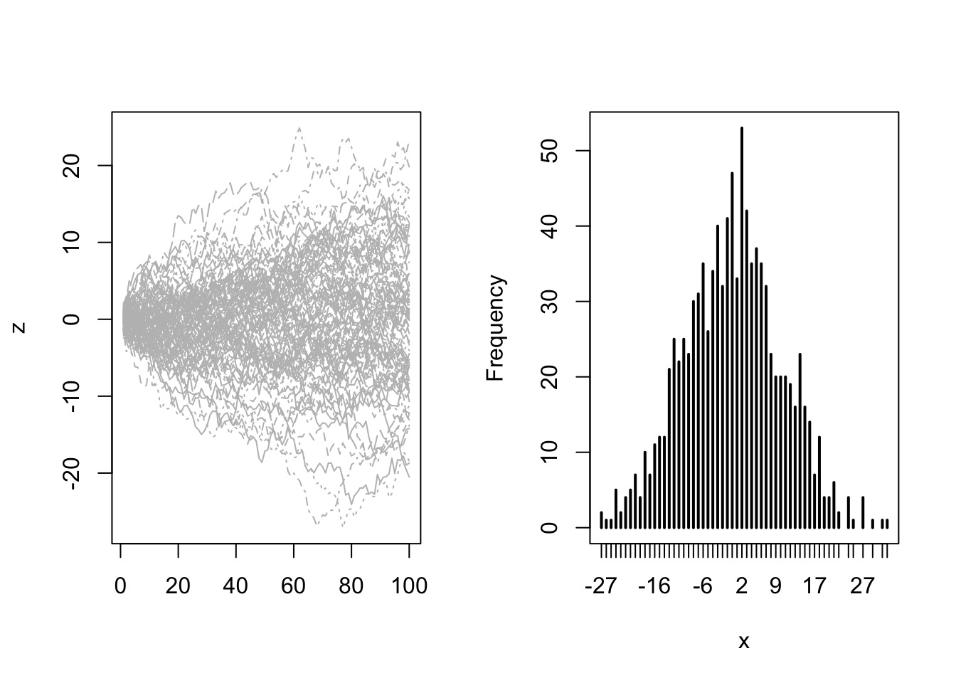
Try it: the Central Limit Theorem
library(rethinking)
simplehist(replicate(10000, sum(rbeta(100,1,1))))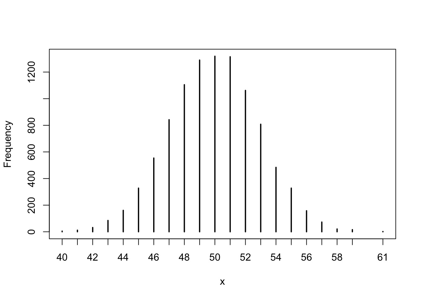
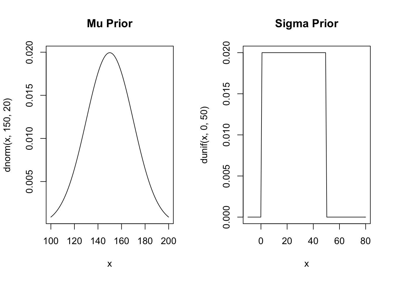
Priors
Posterior
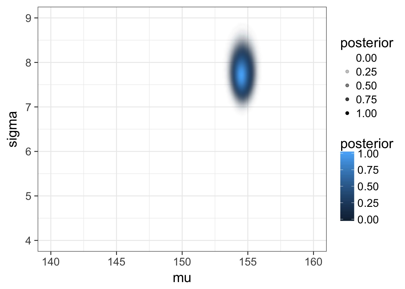
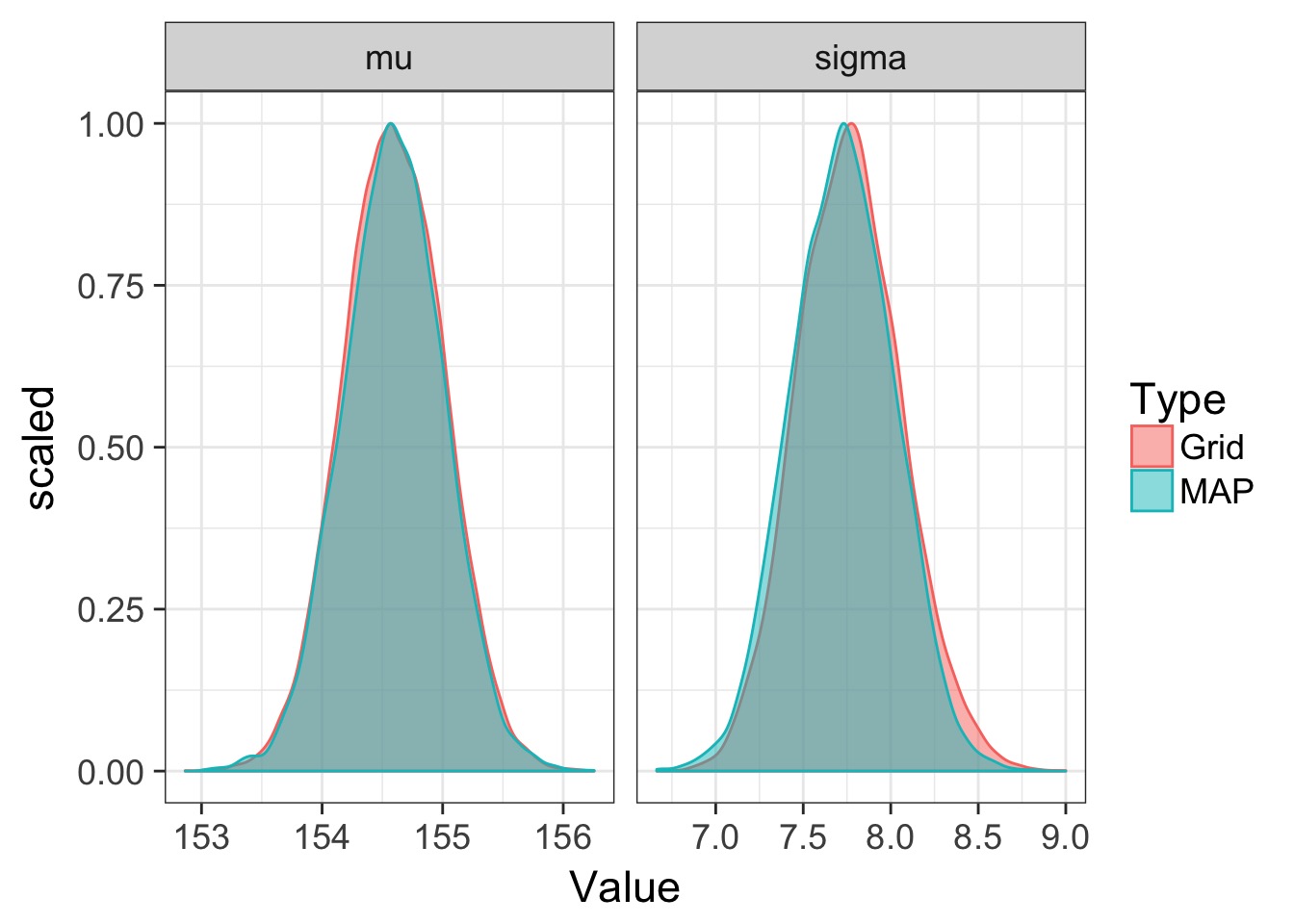
Posterior from a Sample
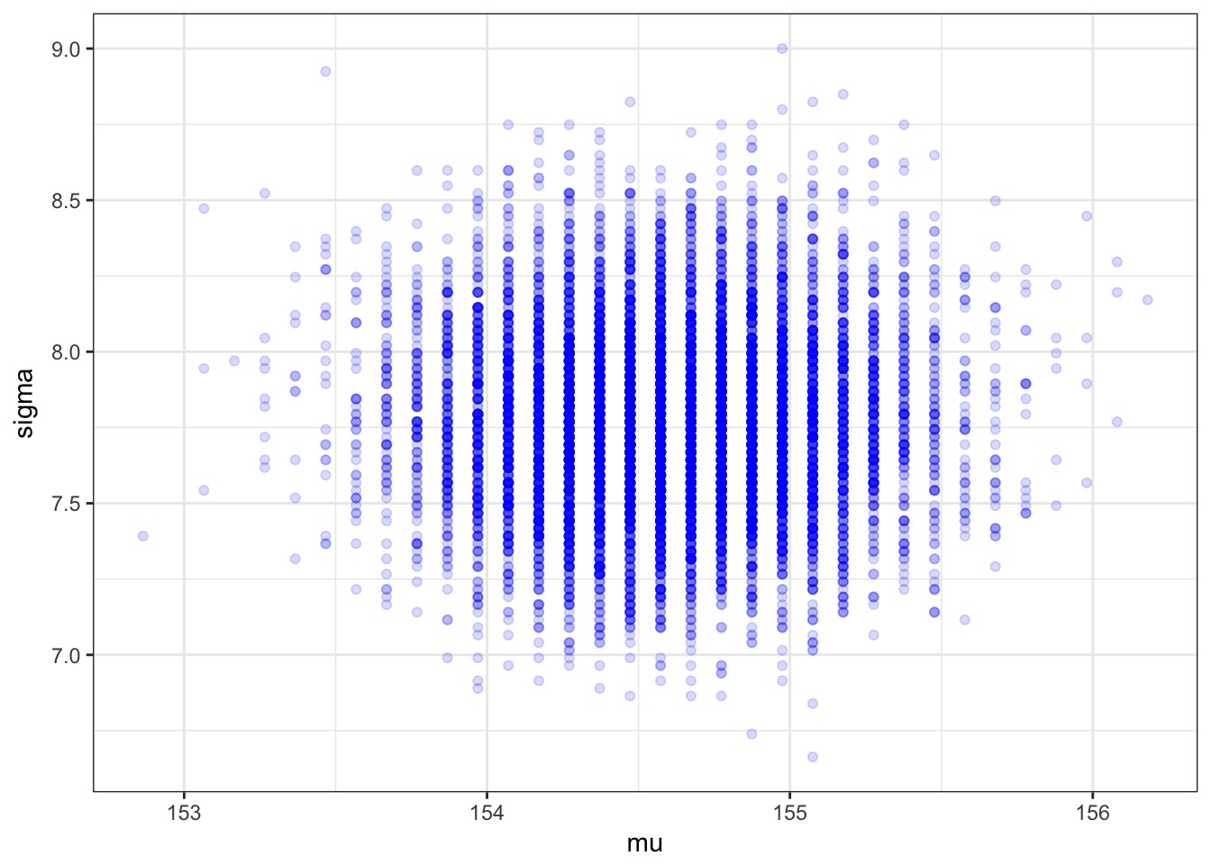
Compare map to grid
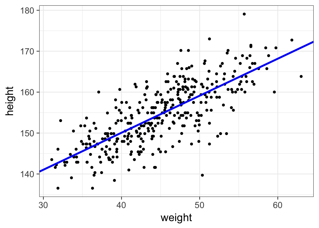
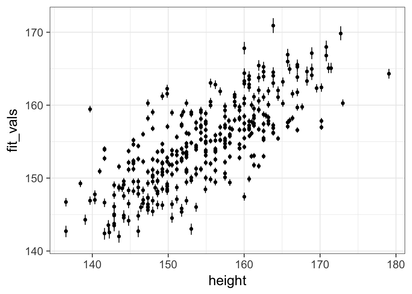
The fit
QQ, etc…
res_vals <- Howell1_Adult$height - fit_vals

qqnorm(res_vals); qqline(res_vals)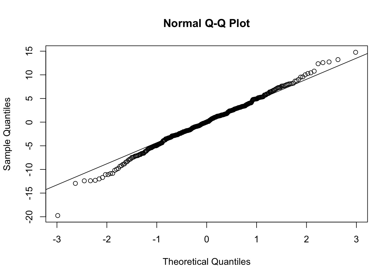
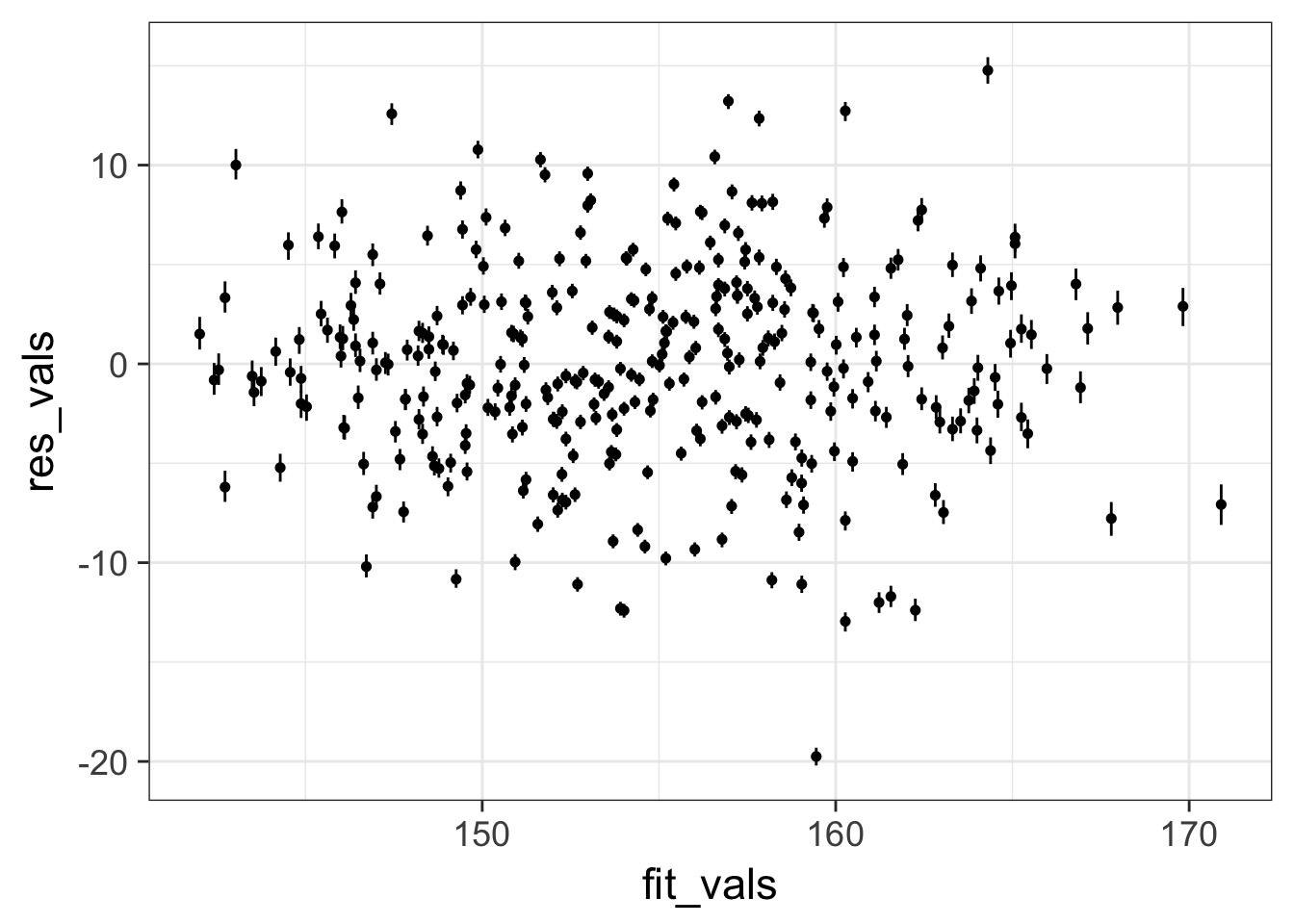
Observed - Fitted
Fit-Residual
Model Results
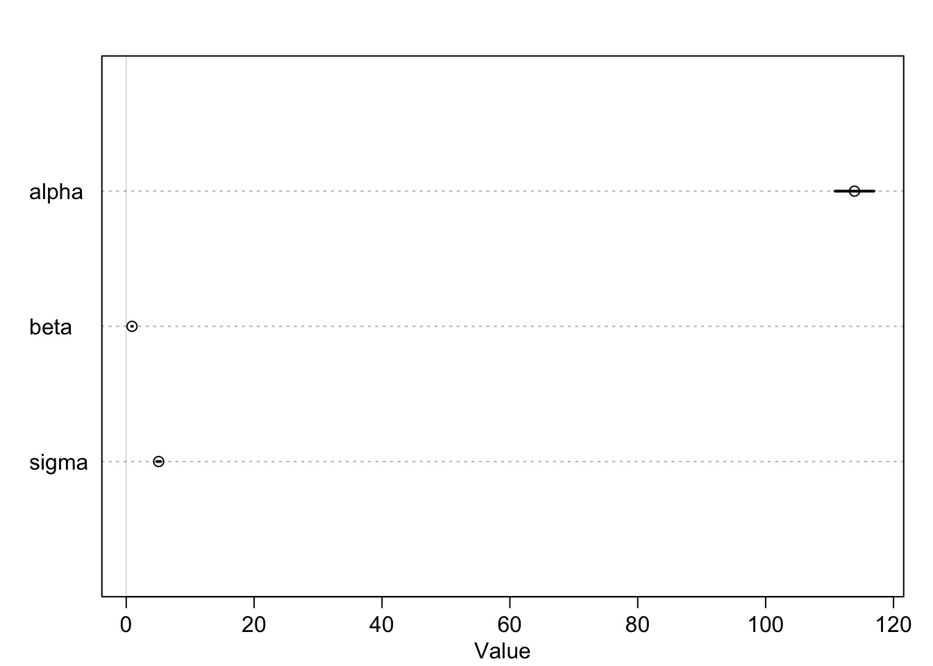
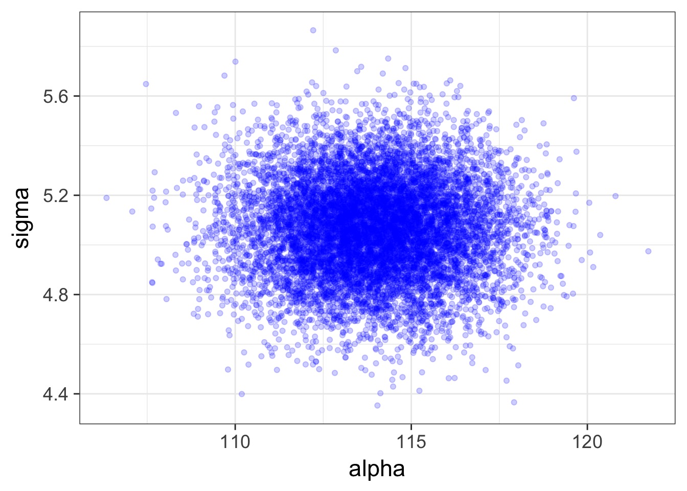
Posterior!
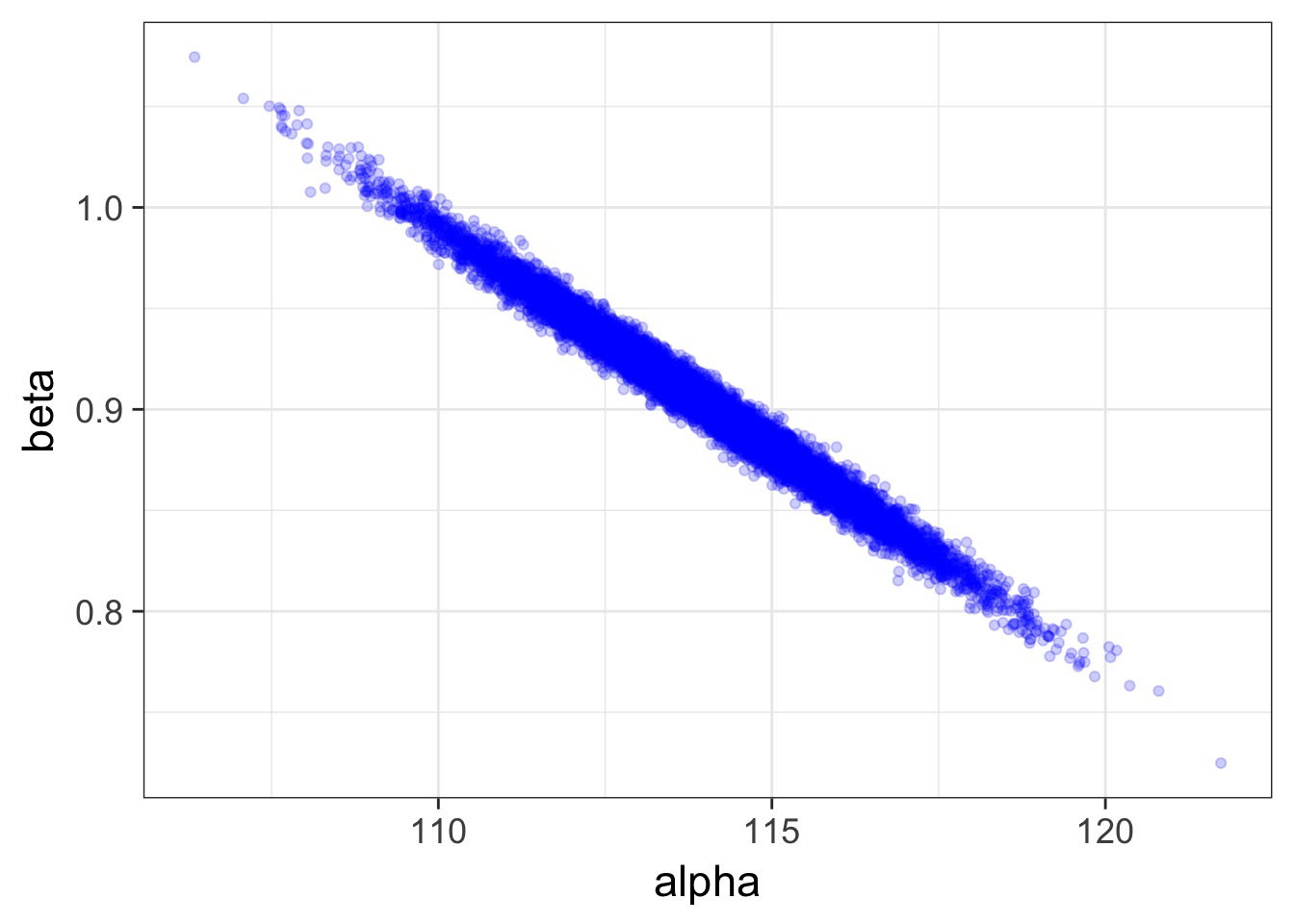
Posterior!
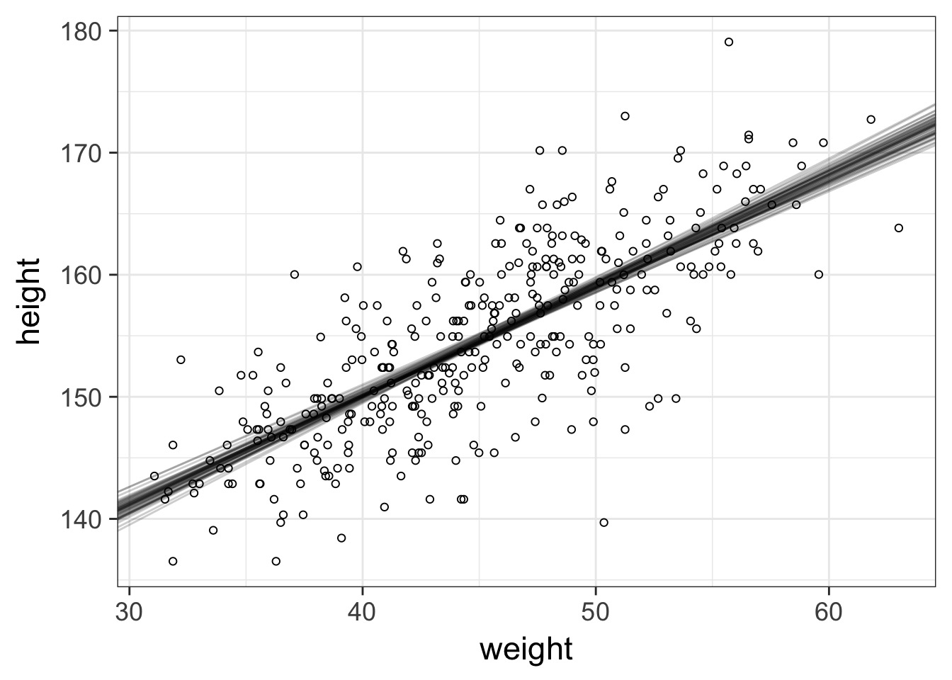
How Well Have we Fit the Data?
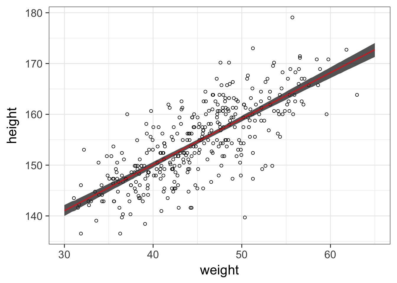
What about with fit intervals?
geom_line and geom_ribbon for plotting
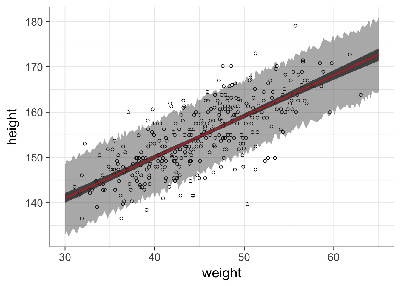
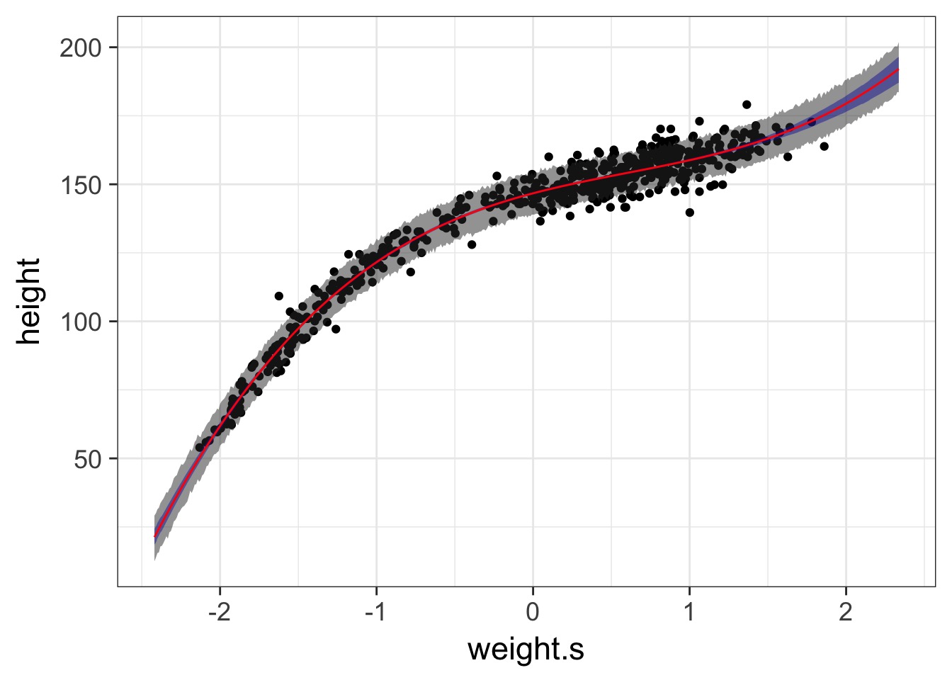
Prediction Interval
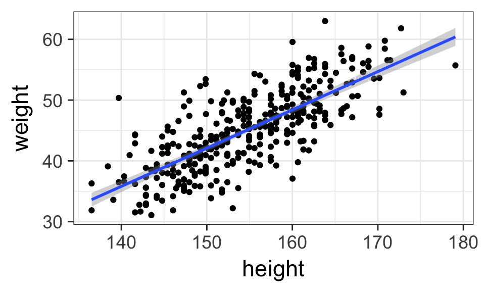
The Actual Data

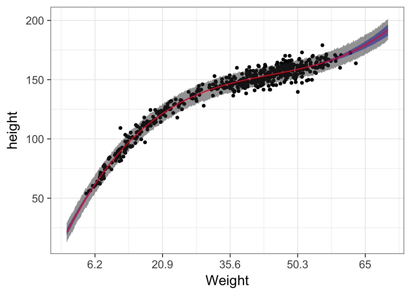
This is not linear
Solution
I hate that x axis
pred_plot +
  scale_x_continuous(label = function(x)
    round(x*sd(Howell1$weight) + mean(Howell1$weight),1)) +
  xlab("Weight")