Our Models Until Now

Likelihood:
\(y_i \sim Normal(\mu_i, \sigma)\)

Data Generating Process
\(\mu_i = \alpha + \beta_1 x1_i + \beta_2 x2_i + ...\)

Priors:
\(\alpha \sim Normal(0, 100)\)
\(\beta_j \sim Normal(0, 100)\)
\(\sigma \sim cauchy(0,2)\)

Making the Normal General

Likelihood:
\(y_i \sim Normal(\mu_i, \sigma)\)

Data Generating Process with identity link
f(\(\mu_i) = \alpha + \beta_1 x1_i + \beta_2 x2_i + ...\)

Priors:
…

A Generalized Linear Model

Likelihood:
\(y_i \sim D(\theta_i, ...)\)

Data Generating Process with identity link
f(\(\theta_i) = \alpha + \beta_1 x1_i + \beta_2 x2_i + ...\)

Priors:
…

The Exponential Family is MaxEnt!

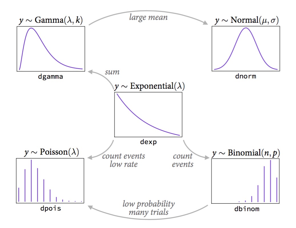
How to determine which non-normal distribution is right for you

• Use previous image to determine
  
  
• Bounded values: binomial, beta
  
  
• Counts: Poisson, multinomial, geometric
  
  
• Distances and durations: exponential, gamma (survival or event history)
  
  
• Monsters: Ranks and ordered categories
  
  
• Mixtures: Beta-binomial, gamma-Poisson, zero- inflated processes

Binomial Logistic Regression

Likelihood:
\(y_i \sim B(size, p_i)\)

Data Generating Process with identity link
logit(\(p_i) = \alpha + \beta_1 x1_i + \beta_2 x2_i + ...\)

Priors:
…

Why Binomial Logistic Regression

• Allows us to predict absolute probability of something occuring
  
  
• Allows us to determing relative change in risk due to predictors

Why a Logit Link?

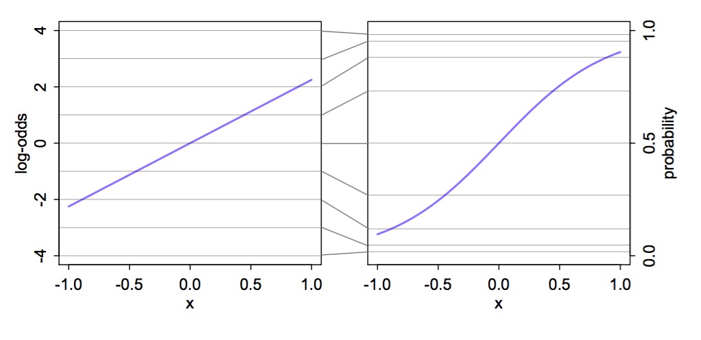
Meaning of Logit Coefficients

\[logit(p_i) = log \frac{p_i}{1-p_i} = \alpha + \beta x_i\]

• \(\frac{p_i}{1-p_i}\) is odds of something happening
  
  
• \(\beta\) is change in log odds per one unit change in \(x_i\)
  • exp(\(\beta\)) is change in odds
    
  • Change in relative risk
    
    
• \(p_i\) is absolute probability of something happening
  • logistic(\(\alpha + \beta x_i\)) = probability
  • To evaluate change in probability, choose two different \(x_i\) values

Binomial GLM in Action: Gender Discrimination in Graduate Admissions

Our data: Berkeley

data(UCBadmit)
head(UCBadmit)

  dept applicant.gender admit reject applications
1    A             male   512    313          825
2    A           female    89     19          108
3    B             male   353    207          560
4    B           female    17      8           25
5    C             male   120    205          325
6    C           female   202    391          593

What model would you build?

  dept applicant.gender admit reject applications
1    A             male   512    313          825
2    A           female    89     19          108
3    B             male   353    207          560
4    B           female    17      8           25
5    C             male   120    205          325
6    C           female   202    391          593

One Model

#female = 1, male = 2
UCBadmit$gender <- as.numeric(UCBadmit$applicant.gender)

mod_gender <- alist(
  #likelihood
  admit ~ dbinom(applications, p),
  
  #Data generating process
  logit(p) <- a[gender],
  
  #priors
  a[gender] ~ dnorm(0,10)
)

fit_gender <- map(mod_gender, UCBadmit)

What do Priors Imply in a GLMS?

#Let's simulate some priors!
prior_sims <- rnorm(1e4, 0, 10)

#back-transformed!
outcomes <- inv_logit(prior_sims)

Visualize what that means!

ggplot(data.frame(outcomes = outcomes),
        aes(x = outcomes)) +
  geom_density()

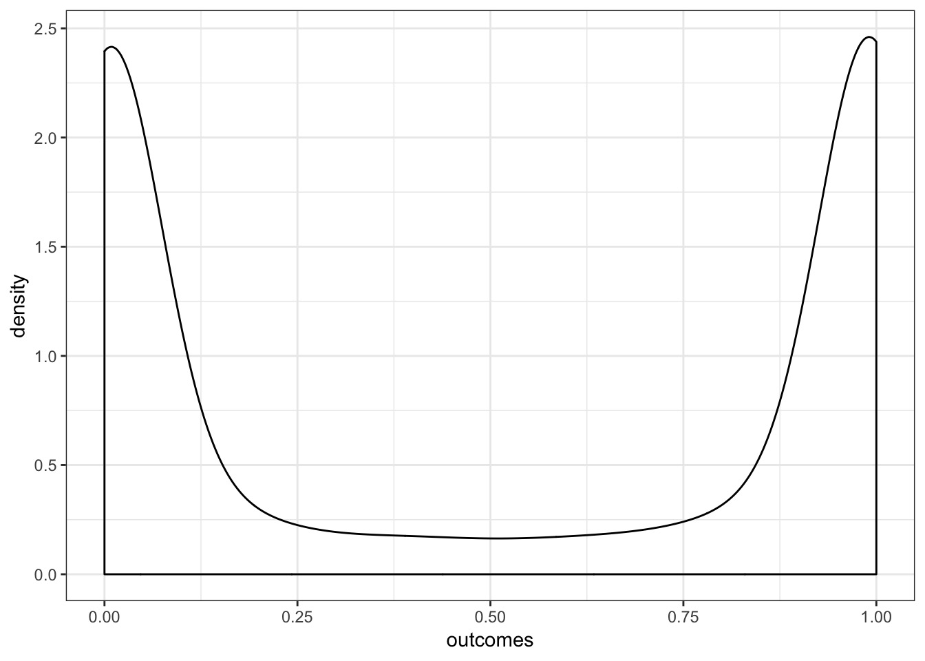
A Flat Prior in Logit Space Might Not Be Flat!

ggplot(data.frame(outcomes = outcomes),
        aes(x = outcomes)) +
  geom_density()

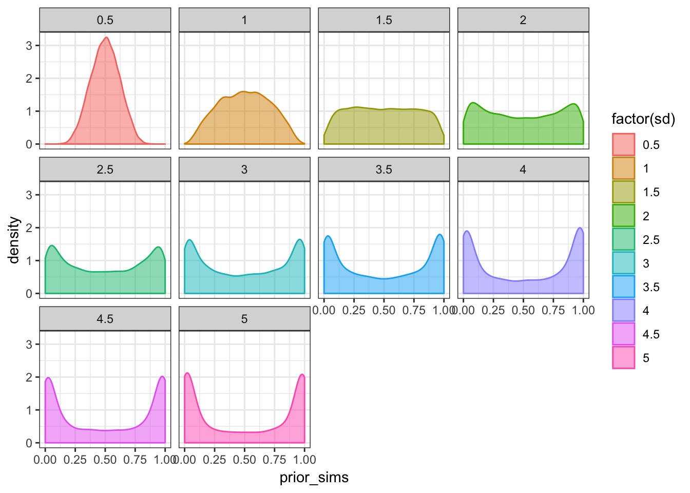
Let’s try a few SDs to see what works!

prior_frame <- tibble(sd = seq(0.5, 5, 0.5)) %>%
  rowwise() %>%
  mutate(prior_sims = list(rnorm(1e4,0,sd))) %>%
  unnest(prior_sims) %>%
  mutate(prior_sims = inv_logit(prior_sims))

What is our flat prior?

A New Model

mod_gender <- alist(
  #likelihood
  admit ~ dbinom(applications, p),
  
  #Data generating process
  logit(p) <- a[gender],
  
  #priors
  a[gender] ~ dnorm(0,1.5)
)

Fit the Model!

fit_gender <- map(mod_gender, UCBadmit)

Results… men do better!

#female = 1, male = 2
precis(fit_gender, depth=2)

      Mean StdDev  5.5% 94.5%
a[1] -0.83   0.05 -0.91 -0.75
a[2] -0.22   0.04 -0.28 -0.16

#Women
logistic(-0.83)

[1] 0.3036451

#Men
logistic(-0.22)

[1] 0.4452208

Relative comparison: Male Advantage

samp <- extract.samples(fit_gender)

exp(mean(samp$a[,2] - samp$a[,1]))

[1] 1.840247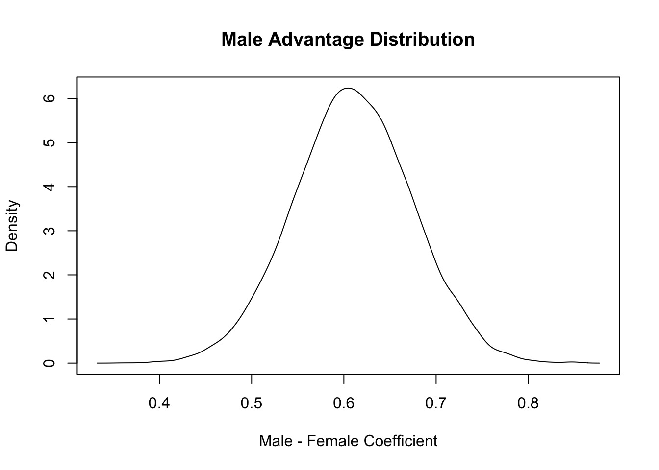

Residuals and Fits

post_pred <- sim(fit_gender)

post_fits <- apply(post_pred, 2, median)

post_res <- sapply(1:nrow(UCBadmit),
              function(i) UCBadmit$admit[i] - post_pred[,i])

res_frame <- tibble(fitted = post_fits, 
                        res = apply(post_res, 2, median),
                        lwr_res = res - apply(post_res, 2, sd),
                        upr_res = res + apply(post_res, 2, sd))

But - can’t use raw residuals

ggplot(res_frame,
       aes(x = fitted, y = res, 
           ymin = lwr_res, ymax = upr_res)) +
  geom_pointrange()

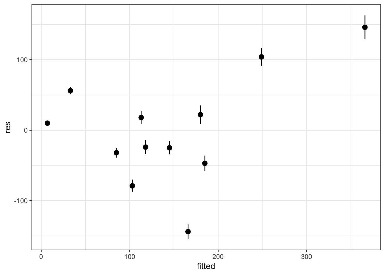
But - can’t use raw residuals

library(tidyr)
res_tib <- as_tibble(post_res) %>%
  gather(variable, value) %>%
  group_by(variable) %>%
  summarize(res = median(value))

ggplot(res_tib, aes(sample = res)) + 
  geom_qq() + geom_qq_line()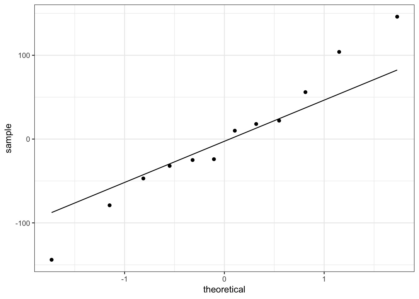

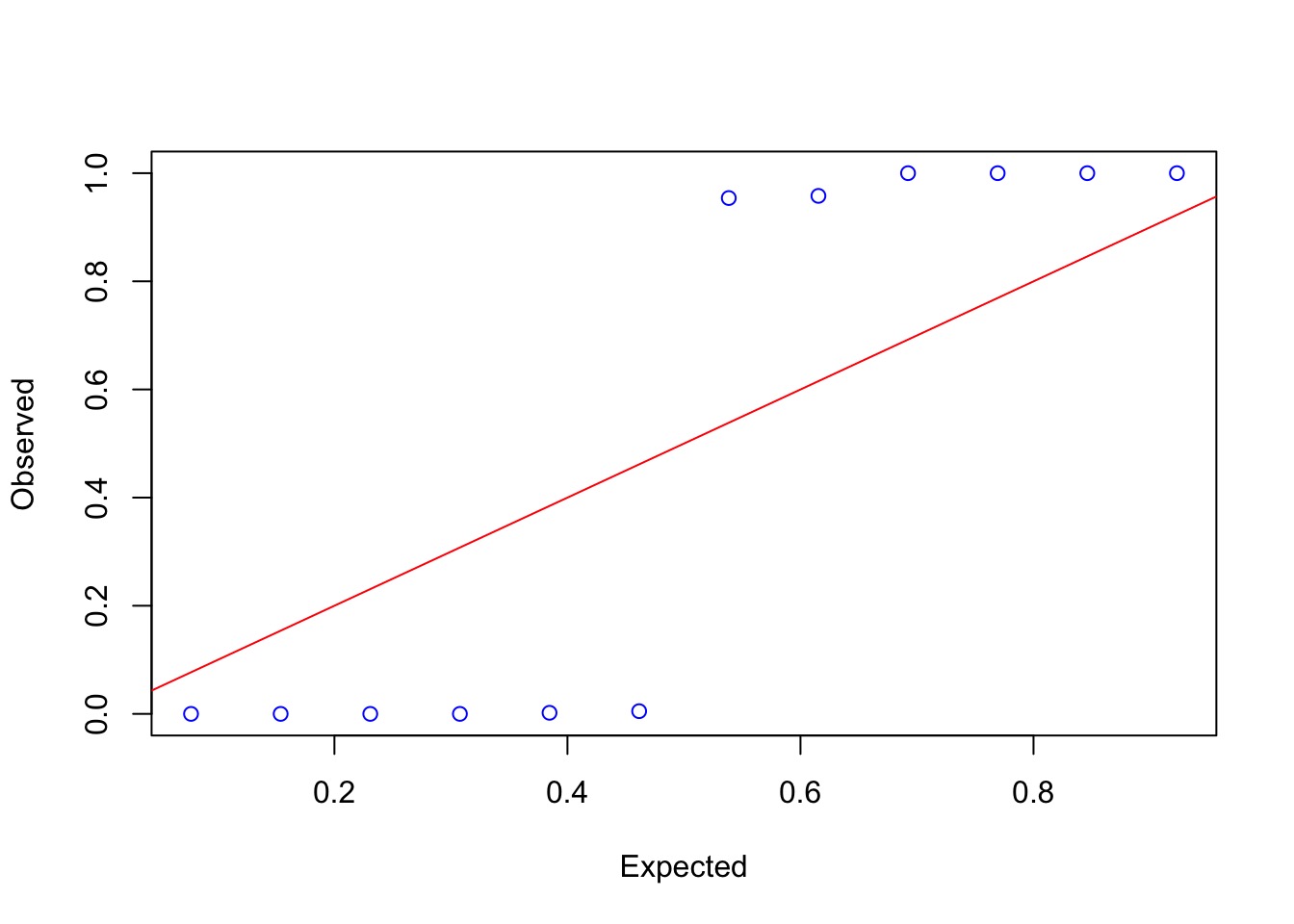
Quantiles of Residuals via Simulation

• Remember that QQ Norm plots don’t work?
  
  
• But we can get quantiles of predictions relative to posterior prediction
  
  
• What % are < the observed value

#figure out how much of each column < observation
quants <- sapply(1:nrow(UCBadmit), function(i){
  
  #what fraction of predictions < the observation
  sum(post_pred[,i] < UCBadmit$admit[i])/nrow(post_pred)
  
})

QQ Unif Looks..not great….

#get the quantiles from the uniform distribution
gap::qqunif(quants, logscale=FALSE)

Why wasn’t this a good model?

postcheck( fit_gender , n=1e4 )

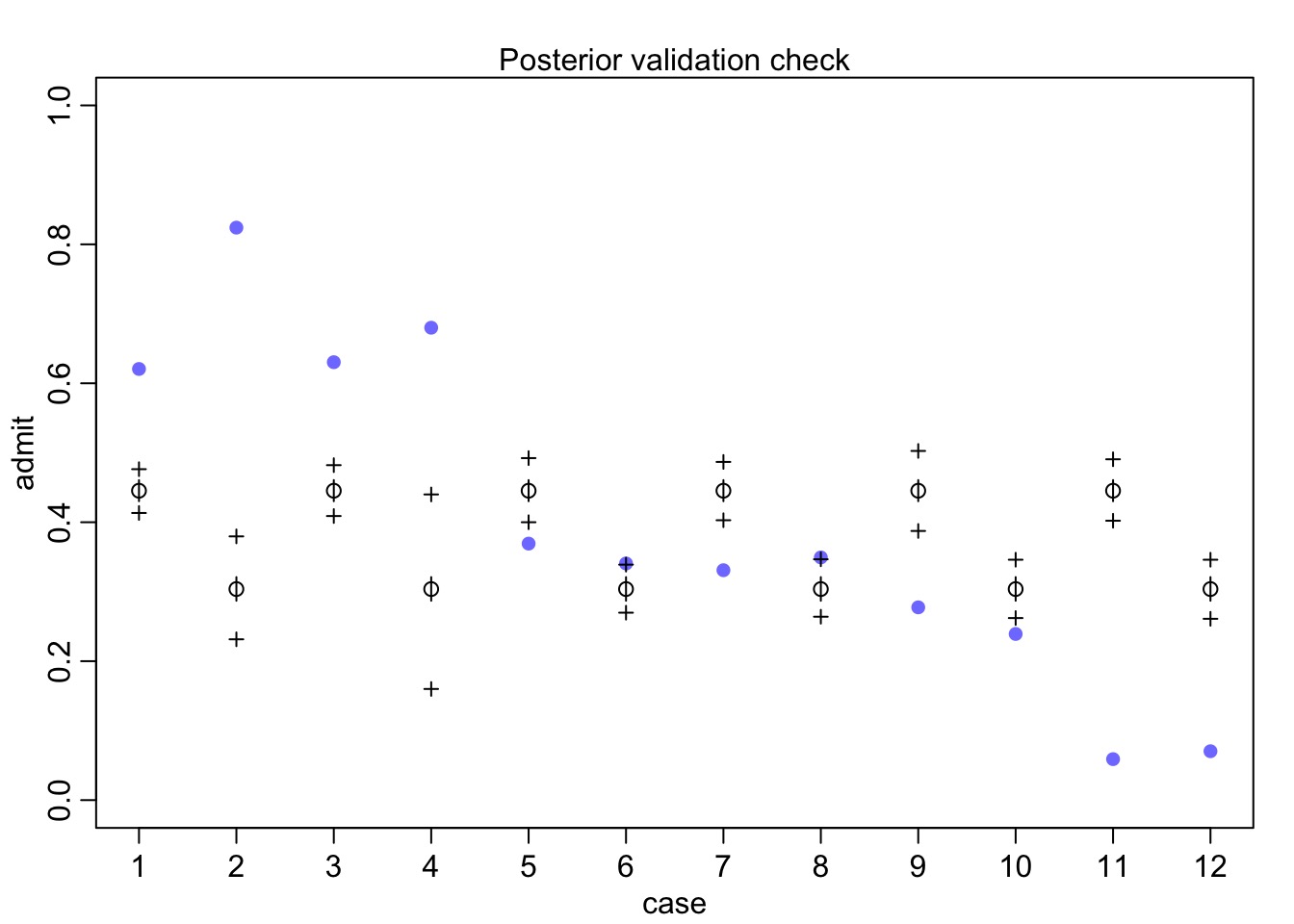
Why wasn’t this a good model?

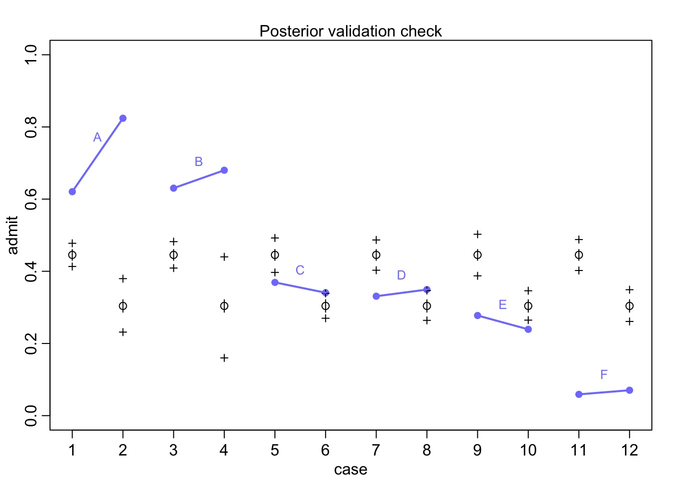
Departments Not Centered on 0 when we consider Department!

UCB_full <- cbind(UCBadmit, res_frame)

ggplot(UCB_full, mapping = aes(x = dept, y = res)) +
  geom_boxplot()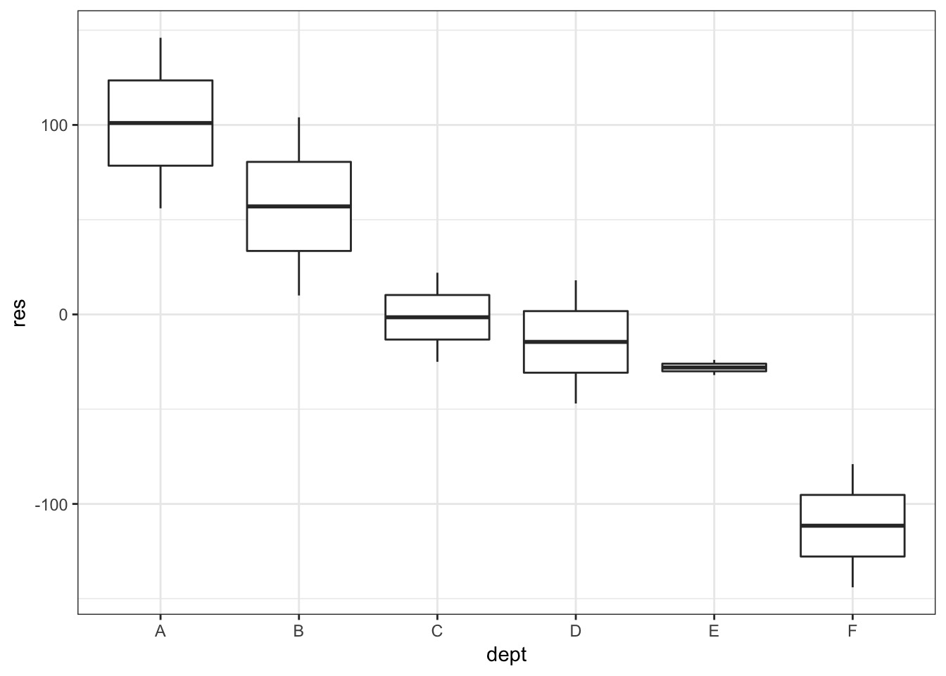

So, department…

#Make a dept index
UCBadmit$dept_id <- as.numeric(UCBadmit$dept)

mod_gender_dept <- alist(
  #likelihood
  admit ~ dbinom(applications, p),
  
  #Data generating process
  logit(p) <- a[dept_id] + b[gender],
  
  #priors
  a[dept_id] ~ dnorm(0,0.5),
  b[gender] ~ dnorm(0,0.5)
)

fit_gender_dept <- map(mod_gender_dept, UCBadmit)

Did it work?

postcheck(fit_gender_dept)

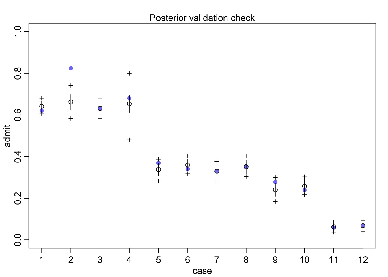
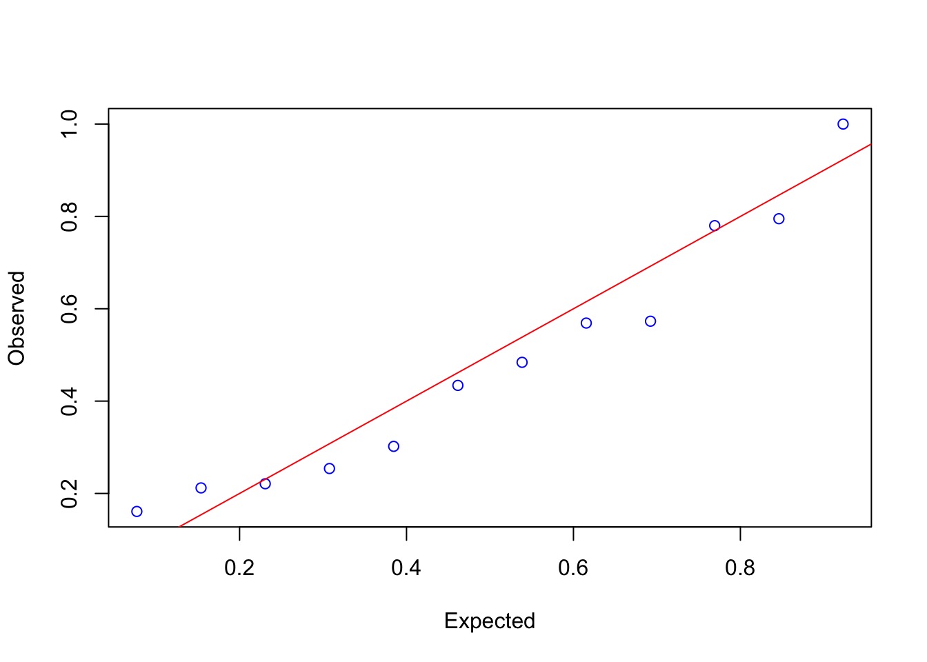
QQ Unif…

#sim gets predictions
post_pred_2 <- sim(fit_gender_dept, refresh=0)

#figure out how much of each column < observation
quants_2 <- sapply(1:nrow(UCBadmit), function(i){
  #what fraction of predictions < the observation
  sum(post_pred_2[,i] < UCBadmit$admit[i])/nrow(post_pred_2)
})

gap::qqunif(quants_2, logscale=FALSE)

Quantile Residuals say Yes!

Outcomes

      Mean StdDev  5.5% 94.5%
a[1]  1.07   0.19  0.76  1.37
a[2]  1.01   0.20  0.70  1.32
a[3] -0.16   0.19 -0.46  0.14
a[4] -0.19   0.19 -0.50  0.11
a[5] -0.62   0.20 -0.93 -0.30
a[6] -2.04   0.21 -2.38 -1.69
b[1] -0.43   0.18 -0.72 -0.13
b[2] -0.50   0.18 -0.79 -0.21

Tool Use and Poisson Regression

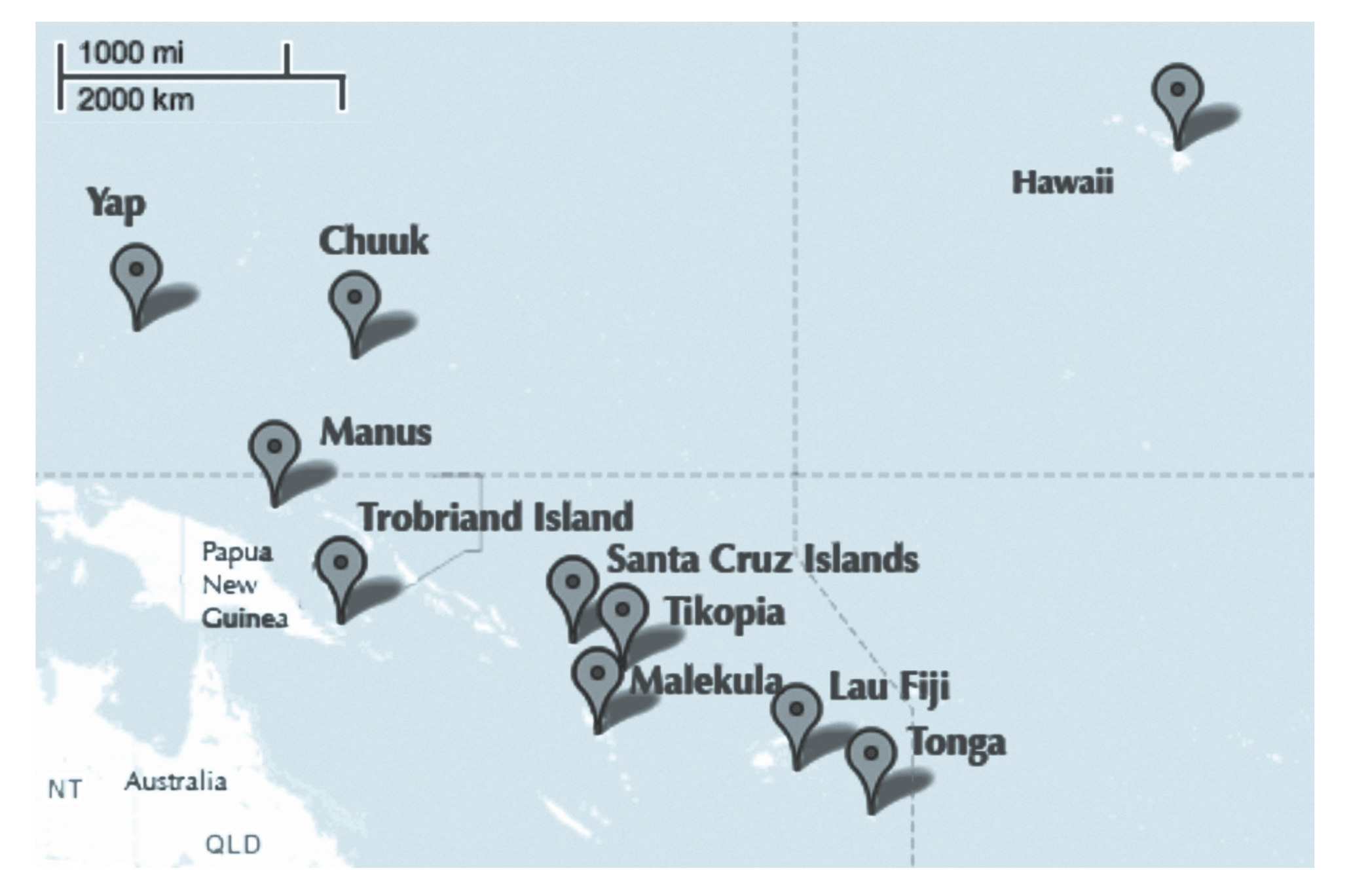
What drives tool use?

     culture population contact total_tools mean_TU
1   Malekula       1100     low          13     3.2
2    Tikopia       1500     low          22     4.7
3 Santa Cruz       3600     low          24     4.0
4        Yap       4791    high          43     5.0
5   Lau Fiji       7400    high          33     5.0
6  Trobriand       8000    high          19     4.0

How to Handle the data?

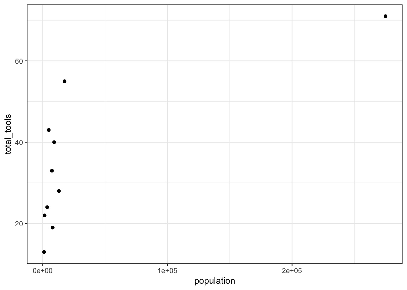
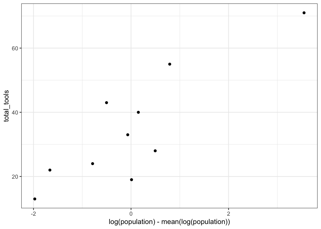
OK, Population scale is off - log it?

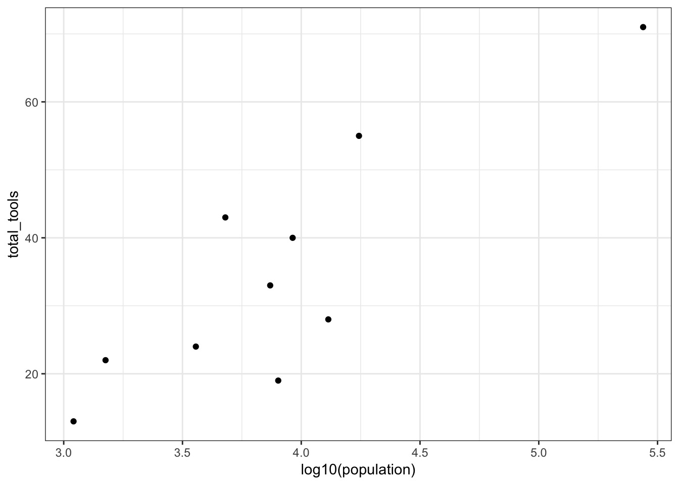
Center Population, as our smallest still have 1K People!

A Simple Model

Kline$P <- log(Kline$population) - mean(log(Kline$population))
  
kline_mod <- alist(
  #likelihood
  total_tools ~ dpois(lambda)
  
  #DGP
  log(lambda) <- a + b * P
  
  #priors
  ...
)

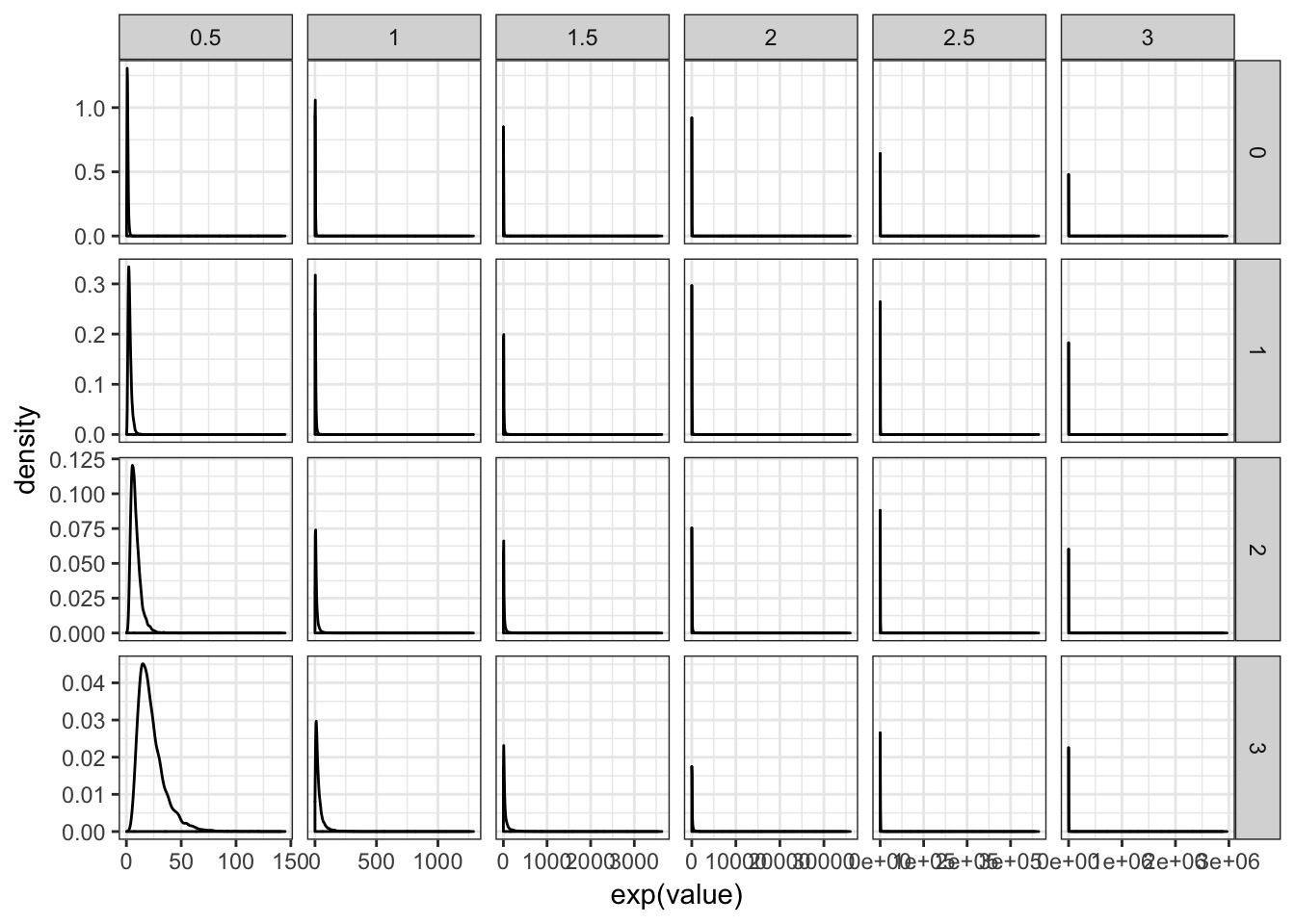
What should our priors be? Data

Try out a few

a_priors <- crossing(m = 0:3, 
                     s = seq(0.5,3,.5)) %>%
  rowwise() %>%
  mutate(value = list(rnorm(1e4, m, s))) %>%
  unnest()

Visualize Priors (data centered on ~40)

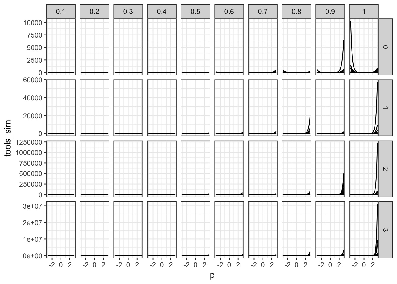
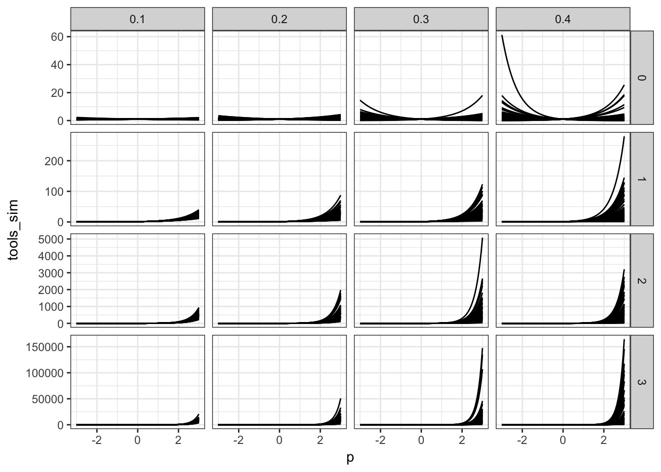
What about b?

b_priors <- crossing(m = 0:3, 
                     s = seq(0.1,1,.1)) %>%
  rowwise() %>%
  mutate(value = list(rnorm(1e2, m, s))) %>%
  unnest() %>%
  
  #make the line
  crossing(p = seq(-3,3, length.out=100)) %>%
  mutate(tools_sim = exp(value*p))

What about b?

What about b?

A Simple Model

Kline$P <- log(Kline$population) - mean(log(Kline$population))

kline_mod <- alist(
  #likelihood
  total_tools ~ dpois(lambda),
  
  #DGP
  log(lambda) <- a + b * P,
  
  #priors
  a ~ dnorm(3,0.5),
  b ~ dnorm(1,0.2)
)

kline_fit <- map2stan(kline_mod, data = Kline)

SAMPLING FOR MODEL 'total_tools ~ dpois(lambda)' NOW (CHAIN 1).
Chain 1: 
Chain 1: Gradient evaluation took 1.4e-05 seconds
Chain 1: 1000 transitions using 10 leapfrog steps per transition would take 0.14 seconds.
Chain 1: Adjust your expectations accordingly!
Chain 1: 
Chain 1: 
Chain 1: Iteration:    1 / 2000 [  0%]  (Warmup)
Chain 1: Iteration:  200 / 2000 [ 10%]  (Warmup)
Chain 1: Iteration:  400 / 2000 [ 20%]  (Warmup)
Chain 1: Iteration:  600 / 2000 [ 30%]  (Warmup)
Chain 1: Iteration:  800 / 2000 [ 40%]  (Warmup)
Chain 1: Iteration: 1000 / 2000 [ 50%]  (Warmup)
Chain 1: Iteration: 1001 / 2000 [ 50%]  (Sampling)
Chain 1: Iteration: 1200 / 2000 [ 60%]  (Sampling)
Chain 1: Iteration: 1400 / 2000 [ 70%]  (Sampling)
Chain 1: Iteration: 1600 / 2000 [ 80%]  (Sampling)
Chain 1: Iteration: 1800 / 2000 [ 90%]  (Sampling)
Chain 1: Iteration: 2000 / 2000 [100%]  (Sampling)
Chain 1: 
Chain 1:  Elapsed Time: 0.017101 seconds (Warm-up)
Chain 1:                0.017591 seconds (Sampling)
Chain 1:                0.034692 seconds (Total)
Chain 1: 

SAMPLING FOR MODEL 'total_tools ~ dpois(lambda)' NOW (CHAIN 1).
Chain 1: 
Chain 1: Gradient evaluation took 6e-06 seconds
Chain 1: 1000 transitions using 10 leapfrog steps per transition would take 0.06 seconds.
Chain 1: Adjust your expectations accordingly!
Chain 1: 
Chain 1: 
Chain 1: WARNING: No variance estimation is
Chain 1:          performed for num_warmup < 20
Chain 1: 
Chain 1: Iteration: 1 / 1 [100%]  (Sampling)
Chain 1: 
Chain 1:  Elapsed Time: 2e-06 seconds (Warm-up)
Chain 1:                1.9e-05 seconds (Sampling)
Chain 1:                2.1e-05 seconds (Total)
Chain 1: 
[ 100 / 1000 ]
[ 200 / 1000 ]
[ 300 / 1000 ]
[ 400 / 1000 ]
[ 500 / 1000 ]
[ 600 / 1000 ]
[ 700 / 1000 ]
[ 800 / 1000 ]
[ 900 / 1000 ]
[ 1000 / 1000 ]

##Did we converge?

plot(kline_fit)

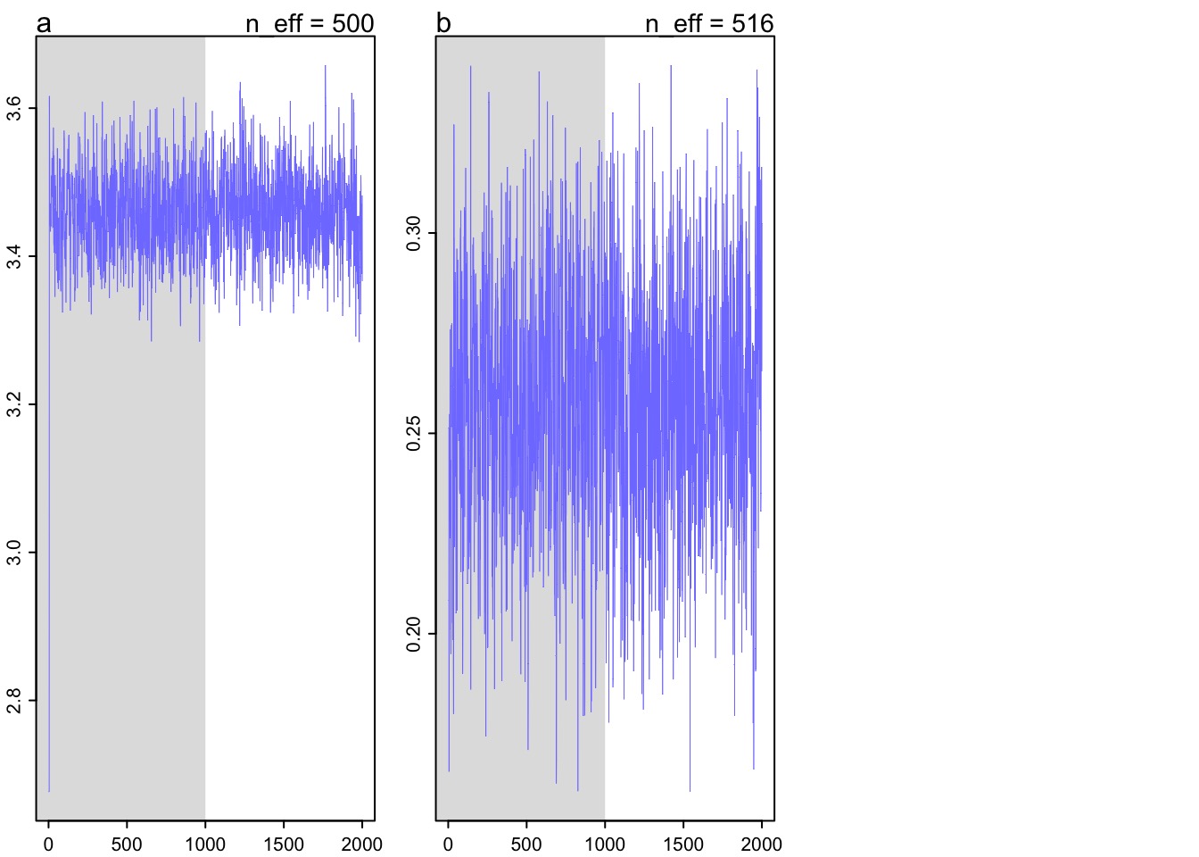
Check your posterior

postcheck(kline_fit)

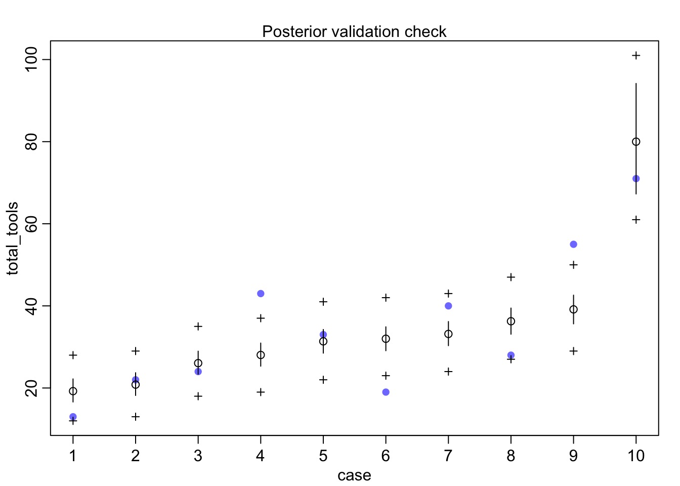
Check Quantile Residuals

#sim gets predictions
kline_post_pred <- sim(kline_fit, refresh=0)

#figure out how much of each column < observation
quants_kline <- sapply(1:nrow(Kline), function(i){
  #what fraction of predictions < the observation
  sum(kline_post_pred[,i] < Kline$total_tools[i])/nrow(kline_post_pred)
})

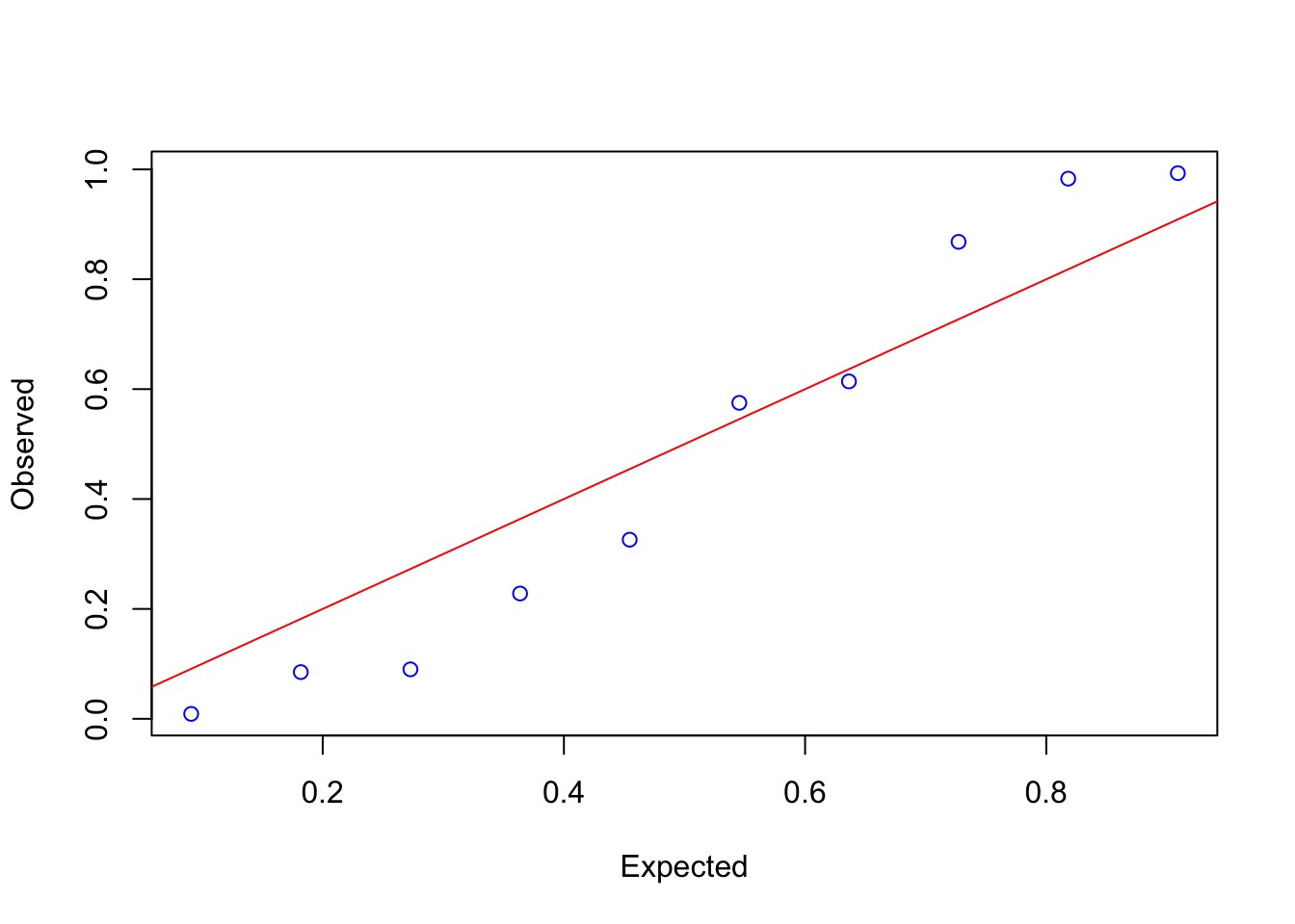
gap::qqunif(quants_kline, logscale=FALSE)

Check Quantile Residuals

Outcomes?

precis(kline_fit)

  Mean StdDev lower 0.89 upper 0.89 n_eff Rhat
a 3.46   0.06       3.37       3.56   500 1.00
b 0.26   0.03       0.21       0.31   516 1.01

Should the link really be linear?

Kline$P <- log(Kline$population) - mean(log(Kline$population))

kline_linear <- alist(
  #likelihood
  total_tools ~ dpois(lambda),
  
  #DGP
  lambda <- a + b * P,
  
  #priors
  a ~ dnorm(3,0.5),
  b ~ dnorm(1,0.2)
)

kline_linear_fit <- map2stan(kline_linear, data = Kline)

SAMPLING FOR MODEL 'total_tools ~ dpois(lambda)' NOW (CHAIN 1).
Chain 1: 
Chain 1: Gradient evaluation took 1.1e-05 seconds
Chain 1: 1000 transitions using 10 leapfrog steps per transition would take 0.11 seconds.
Chain 1: Adjust your expectations accordingly!
Chain 1: 
Chain 1: 
Chain 1: Iteration:    1 / 2000 [  0%]  (Warmup)
Chain 1: Iteration:  200 / 2000 [ 10%]  (Warmup)
Chain 1: Iteration:  400 / 2000 [ 20%]  (Warmup)
Chain 1: Iteration:  600 / 2000 [ 30%]  (Warmup)
Chain 1: Iteration:  800 / 2000 [ 40%]  (Warmup)
Chain 1: Iteration: 1000 / 2000 [ 50%]  (Warmup)
Chain 1: Iteration: 1001 / 2000 [ 50%]  (Sampling)
Chain 1: Iteration: 1200 / 2000 [ 60%]  (Sampling)
Chain 1: Iteration: 1400 / 2000 [ 70%]  (Sampling)
Chain 1: Iteration: 1600 / 2000 [ 80%]  (Sampling)
Chain 1: Iteration: 1800 / 2000 [ 90%]  (Sampling)
Chain 1: Iteration: 2000 / 2000 [100%]  (Sampling)
Chain 1: 
Chain 1:  Elapsed Time: 0.020341 seconds (Warm-up)
Chain 1:                0.016363 seconds (Sampling)
Chain 1:                0.036704 seconds (Total)
Chain 1: 

SAMPLING FOR MODEL 'total_tools ~ dpois(lambda)' NOW (CHAIN 1).
Chain 1: 
Chain 1: Gradient evaluation took 7e-06 seconds
Chain 1: 1000 transitions using 10 leapfrog steps per transition would take 0.07 seconds.
Chain 1: Adjust your expectations accordingly!
Chain 1: 
Chain 1: 
Chain 1: WARNING: No variance estimation is
Chain 1:          performed for num_warmup < 20
Chain 1: 
Chain 1: Iteration: 1 / 1 [100%]  (Sampling)
Chain 1: 
Chain 1:  Elapsed Time: 1e-06 seconds (Warm-up)
Chain 1:                1.9e-05 seconds (Sampling)
Chain 1:                2e-05 seconds (Total)
Chain 1: 
[ 100 / 1000 ]
[ 200 / 1000 ]
[ 300 / 1000 ]
[ 400 / 1000 ]
[ 500 / 1000 ]
[ 600 / 1000 ]
[ 700 / 1000 ]
[ 800 / 1000 ]
[ 900 / 1000 ]
[ 1000 / 1000 ]

Should the link really be linear?

compare(kline_fit, kline_linear_fit)

                  WAIC pWAIC dWAIC weight     SE    dSE
kline_fit         85.6   4.3     0      1   9.39     NA
kline_linear_fit 511.6  17.5   426      0 121.30 123.15

Your turn - What drives tool use?

     culture population contact total_tools mean_TU
1   Malekula       1100     low          13     3.2
2    Tikopia       1500     low          22     4.7
3 Santa Cruz       3600     low          24     4.0
4        Yap       4791    high          43     5.0
5   Lau Fiji       7400    high          33     5.0
6  Trobriand       8000    high          19     4.0