Mixed Models

Today

1. Moving to Mixed Models
   
   
2. Fitting and Evaluating models
   
   
3. Visualizing different types of mixed models
   
   
4. Uncertainty

Random Effects Model

\[Y_{ij} = \alpha_{j} + \epsilon_i\]
\[\alpha_{j} \sim \mathcal{N}(\mu_{\alpha}, \sigma^2_{\alpha})\]
\[\epsilon \sim \mathcal{N}(0, \sigma^2)\]

Now add predictors: Mixed Models with Variable Intercepts

\[Y_{ij} = \alpha_{j} + \beta X_i + \epsilon_i\]
\[\alpha_{j} \sim \mathcal{N}(\mu_{\alpha}, \sigma^2_{\alpha})\]
\[\epsilon \sim \mathcal{N}(0, \sigma^2)\]

Now add predictors: Mixed Models with Variable Slopes

\[Y_{ij} = \alpha + \beta_j X_{ij} + \epsilon_i\]
\[\beta_{j} \sim \mathcal{N}(\mu_{\beta}, \sigma^2_{\beta})\]
\[\epsilon \sim \mathcal{N}(0, \sigma^2)\]

Now add predictors: Mixed Models with Variable Slopes and Intercepts

\[Y_{ij} = \alpha_{ij} + \beta_{j}X_{ij} + \epsilon_{ij}\]

\[\begin{pmatrix} \alpha_{ij} \\ \beta_{ij} \end{pmatrix} \sim \mathcal{MVN}\left ( \begin{pmatrix} \mu_{\alpha} \\ \mu_{\beta} \end{pmatrix} , \begin{pmatrix} \sigma_{\alpha}^{2}& \rho\sigma_{\alpha}\sigma_{\beta}\\ \rho\sigma_{\alpha}\sigma_{\beta} & \sigma_{\beta}^{2} \end{pmatrix} \right )\]
\[\epsilon \sim \mathcal{N}(0, \sigma^2)\]

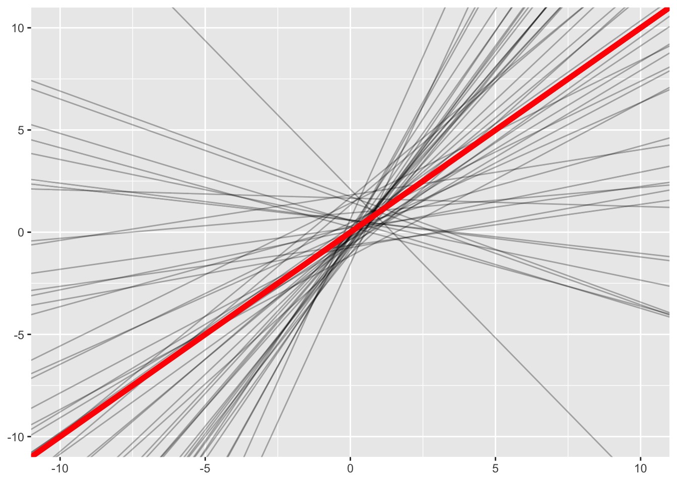
Why MVN?

Today

1. Moving to Mixedl Models
   
2. Fitting and Evaluating models
   
   
3. Visualizing different types of mixed models
   
   
4. Uncertainty

A Greenhouse Experiment testing C:N Ratios

Nesting and Hierarchies

Now add predictors: Mixed Models with Variable Intercepts

\[Y_{ijk} = \alpha_{jk} + \beta X_i + \epsilon_i\]
\[\alpha_{jk} \sim \mathcal{N}(\mu_{\alpha_k}, \sigma^2_{\alpha_j})\]
\[\alpha_{k} \sim \mathcal{N}(\mu_{\alpha}, \sigma^2_{\alpha_k})\]
\[\epsilon \sim \mathcal{N}(0, \sigma^2)\]

Visualizing Our Plant Experiment

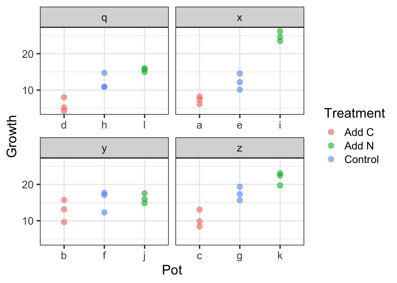
But how variable are things between growth chambers?

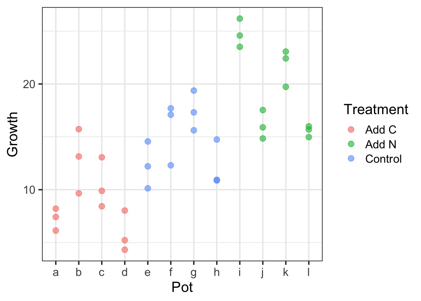
Questions

1. Does treatment matter?
   
   
2. Do we need to account for growth chamber?
   • Note, we at least need to account for non-independence of pot

What random effects do I need to use?

1. Is there a clear and obvious source of non-independence due to a group?
   • Yes, include it!
     
     
     
2. Is there a possible, but, eh, possibly non-problematic source of non-independence?
   • Put it to the test!
     
     

Evaluating Random Effects

• Do this first, as random effect structure alters fixed effects outcomes
  
  
• Use \(\chi^2\) tests for random effects - for a REML fit without any random effects, use gls OR
  
  
• If variance components small, need simulation approaches - see RLRsim

Our Model

plants_mer <- lmer(Growth ~ Treatment +
                     
                  (1|Pot) + (1|Chamber),
                   
                   data= plants)

A Quick Note in Nesting Code

• We did not specify nesting
  
  
• lme4 automagically notes nested structure, calculates random effects appropriately
  
  
• This is not so for nlme - special syntax - 1 | Toplevel / Lowerlevel
  - or 1 | Lowerlevel %in% Toplevel
  
  
• Will work in lme4, but why?

Nesting: These produce equvalent results to plants_mer

`

## LME4
plants_mer2 <- lmer(Growth ~ Treatment +
                     
                  (1|Chamber/Pot) ,
                   
                   data= plants)

## NLME
plants_lme<- lme(Growth ~ Treatment,
                 
                     random = ~ 1|Chamber/Pot,
                 
                     data=plants)

A Test of Random Effects with RLRT

plants_mer_nochamber <- update(plants_mer, . ~ . - (1|Chamber))

anova(plants_mer, plants_mer_nochamber)

Data: plants
Models:
plants_mer_nochamber: Growth ~ Treatment + (1 | Pot)
plants_mer: Growth ~ Treatment + (1 | Pot) + (1 | Chamber)
                     Df    AIC    BIC  logLik deviance  Chisq Chi Df
plants_mer_nochamber  5 185.61 193.53 -87.805   175.61              
plants_mer            6 187.44 196.94 -87.719   175.44 0.1711      1
                     Pr(>Chisq)
plants_mer_nochamber           
plants_mer               0.6791

A Test of Random Effects via Simulation

Need to include a model with ONLY the random effect being tested

library(RLRsim)
        
#No Pot, Only Chamber
plants_mer_only_chamber <- update(plants_mer, . ~ . - (1|Pot))

#The Simulation Test
exactRLRT(m0 = plants_mer_nochamber,
          
          m = plants_mer_only_chamber, 
          
          mA = plants_mer)

A Test of Random Effects via Simulation

Need to include a model with ONLY the random effect being tested

    simulated finite sample distribution of RLRT.
    
    (p-value based on 10000 simulated values)

data:  
RLRT = 0.12832, p-value = 0.2826

Evaluating Random Effects: Final Thoughts

• If your random effect is by design, include it!
  
  
• If you suspect random effects, nature is variable, include them!
  
  
• Carefully consider your RE a priori!
  • Worst case, your design is not sufficient
    
  • In which case, you drop some you cannot estimate
    
  • And/or try alternate fitting methods

Testing fixed effects

• RLRT tests for fixed effects are conservative
  
  
• Provide more weight of Deviance to Random Effects
  
  
• Need to refit models using ML
  - set REML=FALSE

DF for Fixed Effect Testing

• Satterthwaite approximation - Based on sample sizes and variances within groups
  - lmerTest (which is kinda broken at the moment)
  
• Kenward-Roger’s approximation
  - Based on estimate of variance-covariance matrix of fixed effects and a scaling factor
  - More conservative - in car::Anova and pbkrtest

With no Correction

plants_mer_ml <- lmer(Growth ~ Treatment +
                  (1|Pot) + (1|Chamber),
                   data= plants, REML=FALSE)

anova(plants_mer_ml, type = 2)

Analysis of Variance Table
          Df Sum Sq Mean Sq F value
Treatment  2 110.38  55.189  13.559

Note the F test - Chi Sq tests can be biased.

Kenward-Roger Approximation with car::Anova

Anova(plants_mer,  test.statistic="F")

Analysis of Deviance Table (Type II Wald F tests with Kenward-Roger df)

Response: Growth
               F Df Df.res  Pr(>F)  
Treatment 10.172  2      6 0.01181 *
---
Signif. codes:  0 '***' 0.001 '**' 0.01 '*' 0.05 '.' 0.1 ' ' 1

Note that DenDF are 6. Other methods (Satterweith) say 8, lm would have been 33! But only without pot and chamber

Can get Coefficient tests, but…

summary(plants_mer)$coef

                  Estimate Std. Error  t value
(Intercept)       9.102532   1.746777 5.211045
TreatmentAdd N   10.432122   2.312960 4.510291
TreatmentControl  5.301297   2.312960 2.291997

But…Confidence intervals

confint(plants_mer)

                     2.5 %    97.5 %
.sig01           1.3978164  4.598781
.sig02           0.0000000  4.501796
.sigma           1.5578715  2.757033
(Intercept)      5.8670276 12.338023
TreatmentAdd N   5.9984799 14.865782
TreatmentControl 0.8676554  9.734958

confint(plants_mer, method = "Wald")

                     2.5 %    97.5 %
.sig01                  NA        NA
.sig02                  NA        NA
.sigma                  NA        NA
(Intercept)      5.6789128 12.526152
TreatmentAdd N   5.8988038 14.965440
TreatmentControl 0.7679793  9.834616

AIC

• Yes, you can use AIC…carefully
  
  

• Comparison of models with varying fixed effects (marginal AIC) is fine
  
  
• Varying random effects structure…not as much
  
  
• Conditional AIC (cAIC) sensu Vaida and Blanchard 2005 - Uses conditional likelihood and effective DF
  - Based on fit v. observed responses
  - This is an evolving area of research
  
  

• Still gotta do a lot by hand (e.g. cAICc)

cAIC

library(cAIC4)

AIC(plants_mer)

[1] 179.072

cAIC(plants_mer)$caic

[1] 166.6205

cAIC(plants_mer, method="conditionalBootstrap")$caic

[1] 163.1498

cAIC in Action

cAIC(plants_mer)$caic

[1] 166.6205

cAIC(plants_mer)$df

[1] 12.44629

cAIC(plants_mer_nochamber)$caic

[1] 166.2259

cAIC(plants_mer_nochamber)$df

[1] 12.26366

#delta
cAIC(plants_mer_nochamber)$caic - cAIC(plants_mer)$caic

[1] -0.394544

R2

• What does R² mean in the context of mixed models?
  
  
• We are often interested in the explanatory power of fixed effects
  
  
• But random components explain variability in the data
  
  
• We need to decompose these into marginal and conditional R² values - e.g., from fixed and random sources
  
  
• See Schielzeth and Nakagawa 2013 MEE and piecewiseSEM’s implementation

Getting Fit: Marginal v. Conditional R^2

library(piecewiseSEM)

rsquared(plants_mer)

  Response   family     link method  Marginal Conditional
1   Growth gaussian identity   none 0.5556837   0.8787641

rsquared(plants_mer_nochamber)

  Response   family     link method  Marginal Conditional
1   Growth gaussian identity   none 0.5556466   0.8787815

Get Treatment Estimates from emmeans

library(emmeans)
trt_means <- emmeans(plants_mer, specs = ~Treatment)

trt_means

 Treatment emmean   SE   df lower.CL upper.CL
 Add C        9.1 1.75 8.73     5.13     13.1
 Add N       19.5 1.75 8.73    15.56     23.5
 Control     14.4 1.75 8.73    10.43     18.4

Degrees-of-freedom method: kenward-roger 
Confidence level used: 0.95 

Posthocs from emmeans

contrast(trt_means, "pairwise")

 contrast        estimate   SE df t.ratio p.value
 Add C - Add N     -10.43 2.31  6 -4.510  0.0097 
 Add C - Control    -5.30 2.31  6 -2.292  0.1331 
 Add N - Control     5.13 2.31  6  2.218  0.1462 

P value adjustment: tukey method for comparing a family of 3 estimates 

So, what was different?

• Maybe you want to look at random effects structure?
  
  
• Diagnostics are still key!
  
  
• You can be fiddly with tests, or…
   
• You can evaluate model implications with posthoc simulations of predictions!!

Today

1. Brief review
   
   
2. Evaluating models
   
   
3. Visualizing different types of mixed models
   
   
4. Uncertainty

Types of Mixed Models

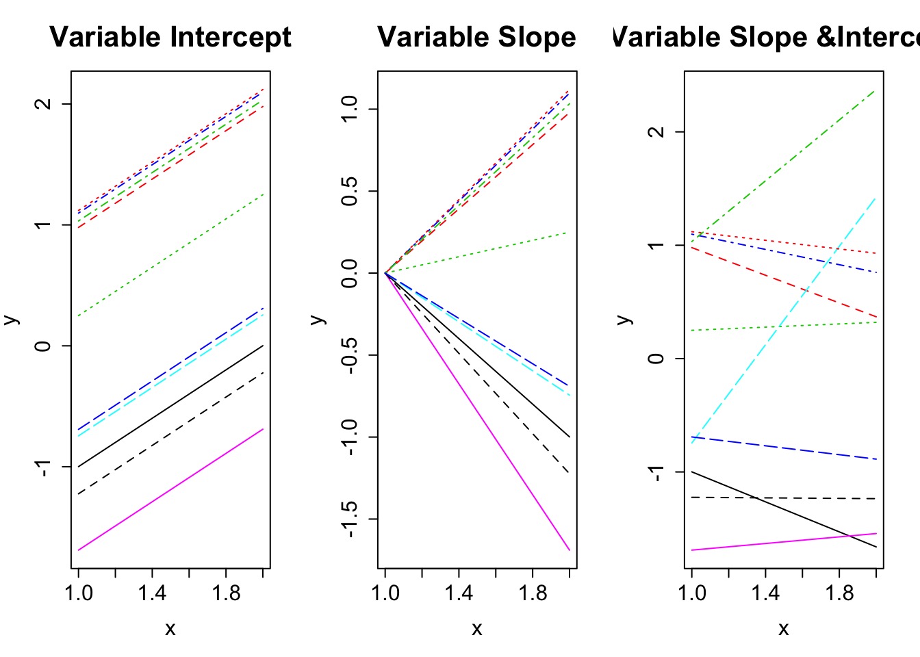
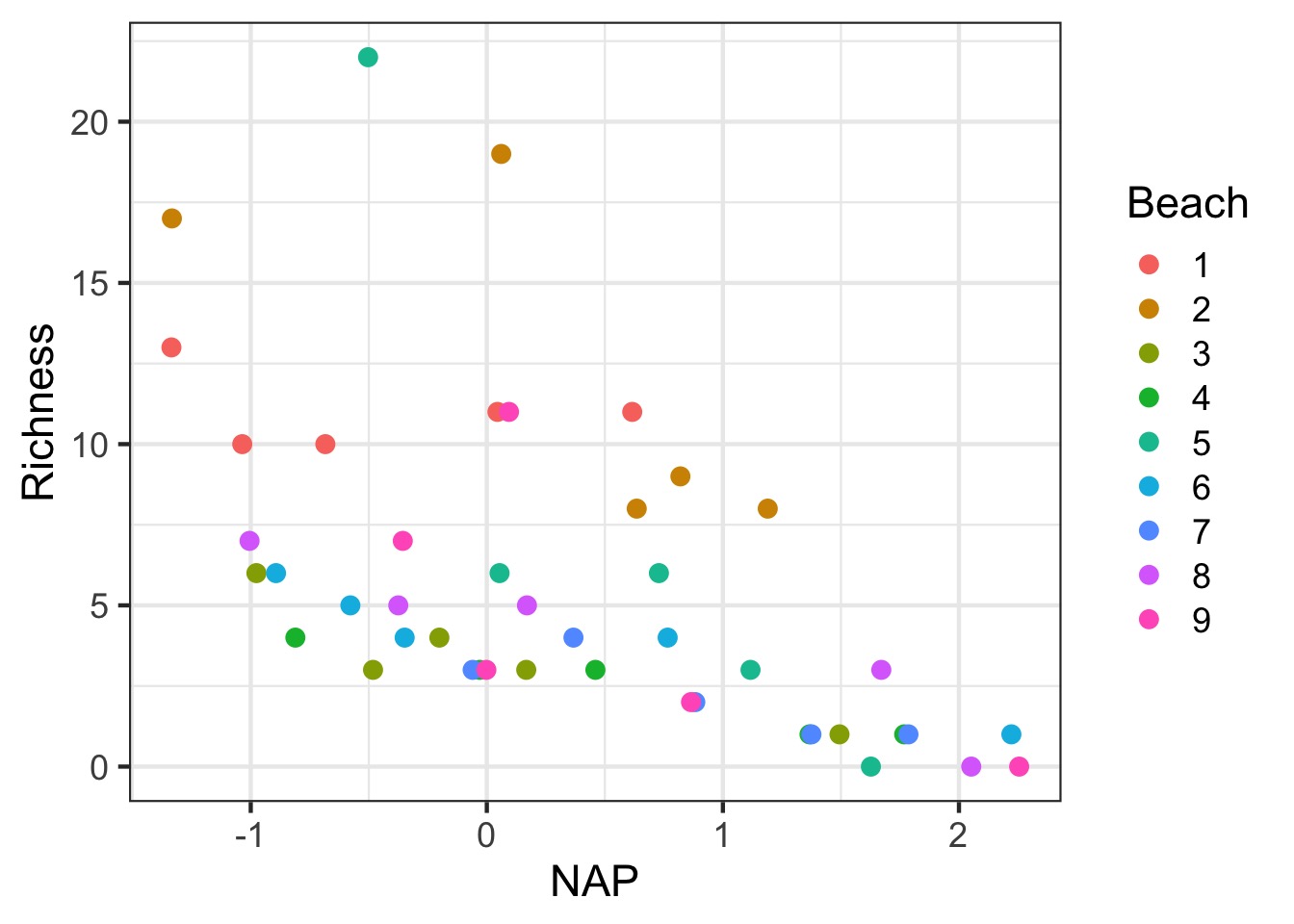
Let’s take this to the beach with Tide Height

We’ve seen a Variable Intercept Model Already

rikz <- read.csv("./data/08/rikz.csv")
rikz$Beach <- factor(rikz$Beach) #it was continuous


rikz_varint <- lmer(Richness ~ NAP + (1|Beach), 
                    data=rikz)

How to Plot?

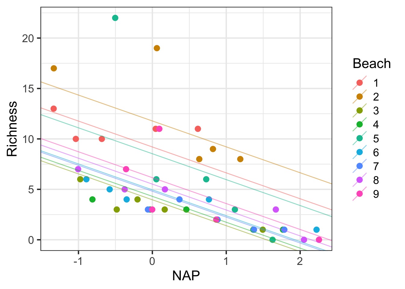
Adding Variable Intercepts

rikz_varint_lines <- coef(rikz_varint)$Beach
rikz_varint_lines$Beach <- levels(rikz$Beach)

rikz_plot <- rikz_plot_base +
  geom_abline(data=rikz_varint_lines,
              aes(slope = NAP, intercept=`(Intercept)`, 
                  color=Beach),
              alpha=0.5)

rikz_plot

Adding Variable Intercepts

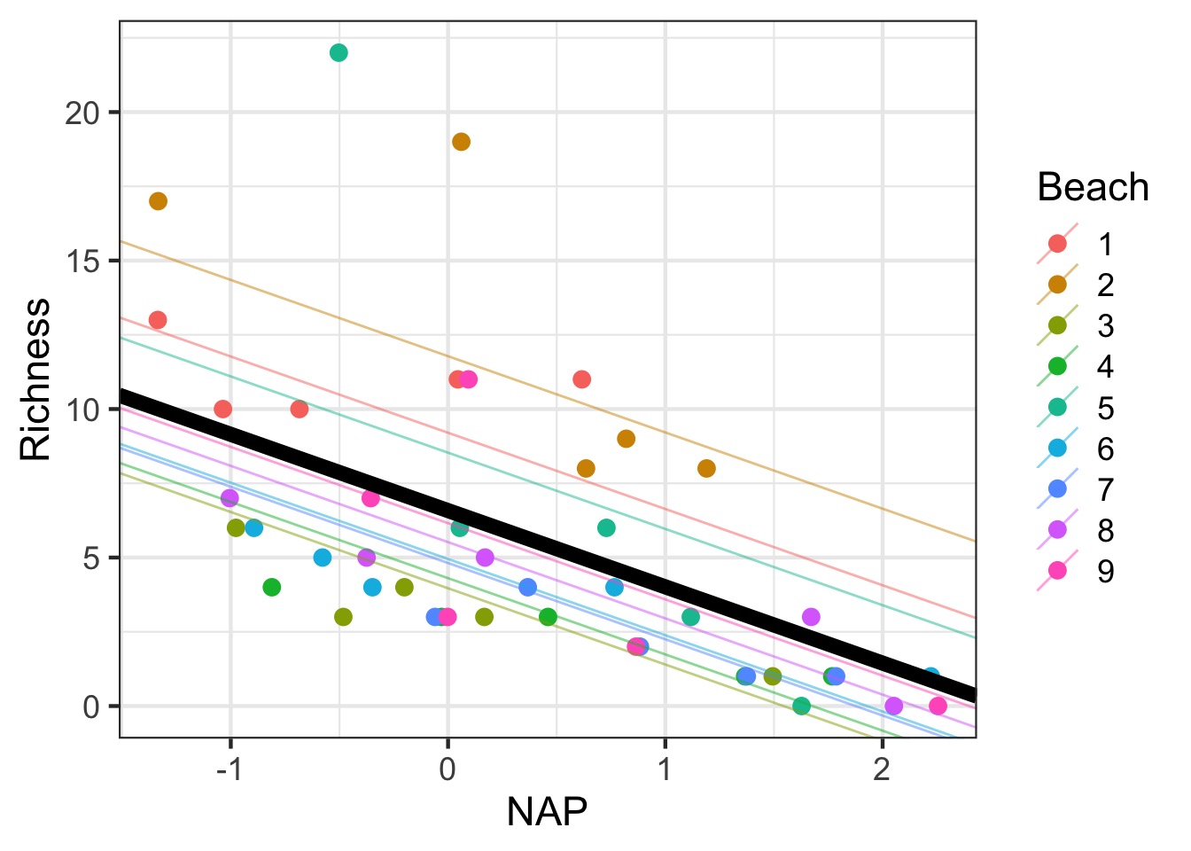
Adding the fixed effect

rikz_plot +
  geom_abline(slope=fixef(rikz_varint)[2],
              intercept=fixef(rikz_varint)[1],
              size=3)

Adding the fixed effect

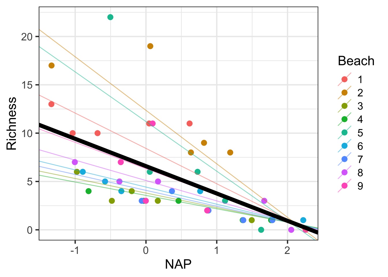
Variable Slope Model

\[Y_{ij} = \alpha + \beta_j X_{ij} + \epsilon_i\]
\[\beta_{j} \sim \mathcal{N}(\mu_{\beta}, \sigma^2_{\beta})\]
\[\epsilon \sim \mathcal{N}(0, \sigma^2)\]

Variable Slope Model

rikz_varslope <- lmer(Richness ~ NAP + 
                        
                        (NAP - 1|Beach), 
                      
                      
                    data=rikz)

Note the - 1 to denote only the slope is varying

Variable Slope-Intercept Model

\[Y_{ij} = \alpha_{ij} + \beta_{j}X_{ij} + \epsilon_{ij}\]

\[\begin{pmatrix} \alpha_{ij} \\ \beta_{ij} \end{pmatrix} \sim \mathcal{MVN}\left ( \begin{pmatrix} \mu_{\alpha} \\ \mu_{\beta} \end{pmatrix} , \begin{pmatrix} \sigma_{\alpha}^{2}& \rho\sigma_{\alpha}\sigma_{\beta}\\ \rho\sigma_{\alpha}\sigma_{\beta} & \sigma_{\beta}^{2} \end{pmatrix} \right )\]
\[\epsilon \sim \mathcal{N}(0, \sigma^2)\]

Variable Slope-Intercept Model

#Note use of different optimizer!
rikz_varslopeint <- lmer(Richness ~ NAP + 
                           
                           (NAP + 1|Beach), 
                         
                         data=rikz,
                         
                         control=lmerControl(optimizer="bobyqa"))

Variable Slope Intercept Model

Which Random Effects do I need - Look at al of those variances!

Testing Variable Intercept structure

#refit = FALSE as anova defaults to refitting models with REML=FALSE
anova(rikz_varslopeint, rikz_varslope, refit=FALSE)

Data: rikz
Models:
rikz_varslope: Richness ~ NAP + (NAP - 1 | Beach)
rikz_varslopeint: Richness ~ NAP + (NAP + 1 | Beach)
                 Df    AIC    BIC  logLik deviance  Chisq Chi Df
rikz_varslope     4 260.20 267.43 -126.10   252.20              
rikz_varslopeint  6 244.38 255.22 -116.19   232.38 19.817      2
                 Pr(>Chisq)    
rikz_varslope                  
rikz_varslopeint  4.975e-05 ***
---
Signif. codes:  0 '***' 0.001 '**' 0.01 '*' 0.05 '.' 0.1 ' ' 1

Testing Variable Slope structure

anova(rikz_varslopeint, rikz_varint, refit=FALSE)

Data: rikz
Models:
rikz_varint: Richness ~ NAP + (1 | Beach)
rikz_varslopeint: Richness ~ NAP + (NAP + 1 | Beach)
                 Df    AIC    BIC  logLik deviance  Chisq Chi Df
rikz_varint       4 247.48 254.71 -119.74   239.48              
rikz_varslopeint  6 244.38 255.22 -116.19   232.38 7.0964      2
                 Pr(>Chisq)  
rikz_varint                  
rikz_varslopeint    0.02878 *
---
Signif. codes:  0 '***' 0.001 '**' 0.01 '*' 0.05 '.' 0.1 ' ' 1

Today

1. Brief review
   
   
2. Evaluating models
   
   
3. Visualizing different types of mixed models
   
   
4. Uncertainty

Plotting Uncertainty in Fixed Effects via Simulation

library(merTools)
#The fit values
predDF <- predictInterval(rikz_varslopeint,
                          newdata=rikz,
                          which="fixed",
                          include.resid.var = FALSE)
predDF$NAP <- rikz$NAP

Plotting Uncertainty via Simulation

#The Plot
rikz_plot_base +
  geom_abline(slope=fixef(rikz_varslopeint)[2],
              intercept=fixef(rikz_varslopeint)[1],
              size=2.5, color="blue") +
  geom_ribbon(data=predDF, mapping=aes(y = fit, ymin=lwr, ymax=upr), 
              alpha=0.3, color="grey")

Plotting Uncertainty via Simulation

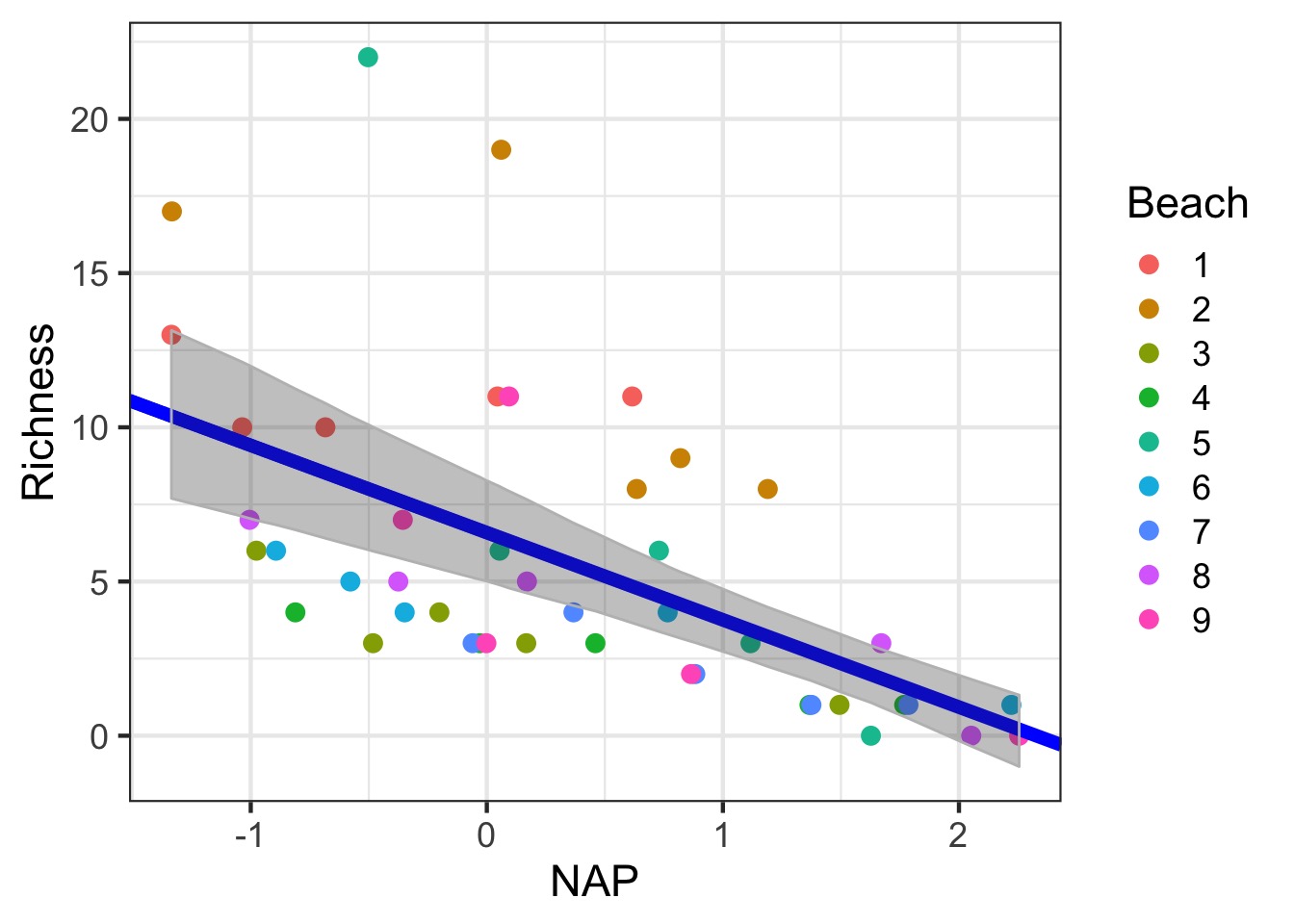
Showing Fixed Prediction Uncertainty: include.resid.var=TRUE

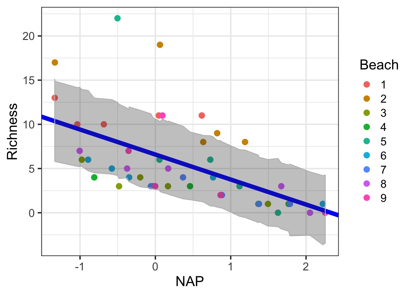
Getting the Uncertainty due to Random Effects: Generalization

#new data for all beaches
uncDF <- data.frame(expand.grid(Beach = levels(rikz$Beach),
                    NAP = seq(min(rikz$NAP), max(rikz$NAP), 
                                                 length.out=200)))

#fit values
pred_re_df <- predictInterval(rikz_varslopeint,
                          newdata=uncDF,
                          which="full",
                          include.resid.var = FALSE)

#get the wide range
fit_re_df <- cbind(uncDF, pred_re_df) %>%
  group_by(NAP) %>%
  summarize(fit=mean(fit), lwr = min(lwr), upr = max(upr)) %>%
  ungroup()

Fit and Random Error

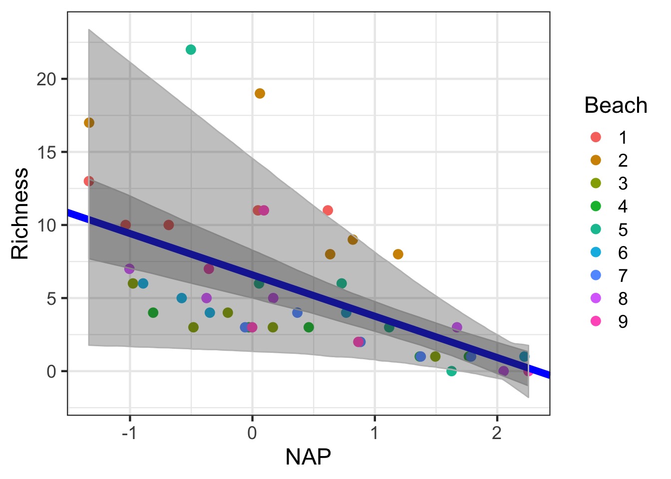
Getting the Full Range of Uncertainty

#fit values with full uncertainty
pred_unc_df <- predictInterval(rikz_varslopeint,
                          newdata=uncDF,
                          which="full",
                          include.resid.var = TRUE)

#get the wide range
fit_unc_df <- cbind(uncDF, pred_unc_df) %>%
  group_by(NAP) %>%
  summarize(fit=mean(fit), lwr = min(lwr), upr = max(upr)) %>%
  ungroup()

Getting the Full Range of Uncertainty

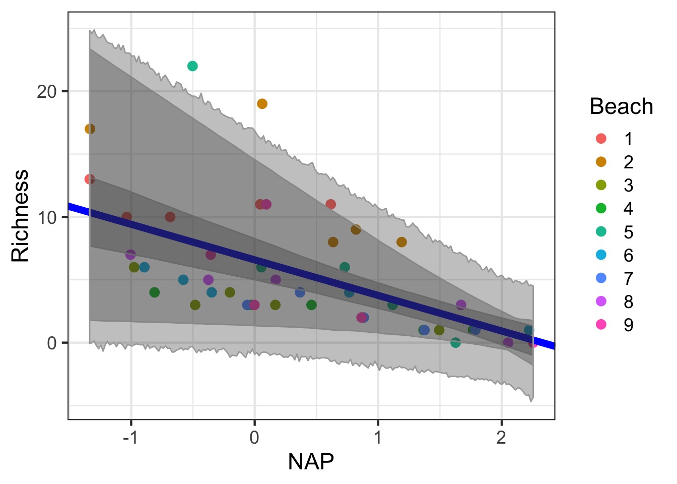
Need all three for extrapolation

Example

• Load up the RIKZ data
  
  
• Look at both exposure and NAP
  
  
• Test fixed and random effects
  
  
• Visualize results

General Protocol for Model Fitting

1. Start with model with all fixed and random effects that may be important. Evaluate with diagnostics.
   
   
2. Evaluate random effects with full model of all fixed effects using REML(\(\chi^2\), RLRT, cAIC, etc.)
   
   
3. Evaluate fixed effects with reduced random effects (F Tests using ML fit)
   
   
4. Model diagnostics again…
   
   
5. Draw inference from model using Wald tests, lsmeans, visualization, etc.