Taking Least Squares From the Ordinary to the General(ized)

Basic Princples of Ordinary Least Squares

Y is determined by X: p(Y \(|\) X=x)
The relationship between X and Y is Linear
The residuals of \(\widehat{Y_i} = \beta_0 + \beta_1 X_i + \epsilon\) are normally distributed
(i.e., \(\epsilon_i \sim\) N(0,\(\sigma\)))

Basic Principles of Ordinary Least Squares

\(\widehat{Y} = \beta_0 + \beta_1 X + \epsilon\) where \(\beta_0\) = intercept, \(\beta_1\) = slope

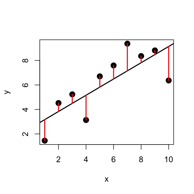
Minimize Residuals defined as \(SS_{residuals} = \sum(Y_{i} - \widehat{Y})^2\)

But…what about this?

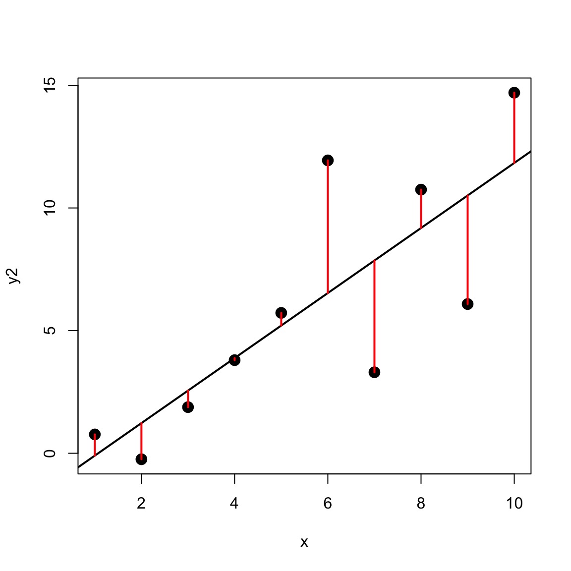
Variance-Mean Relationship

Or…what about this?

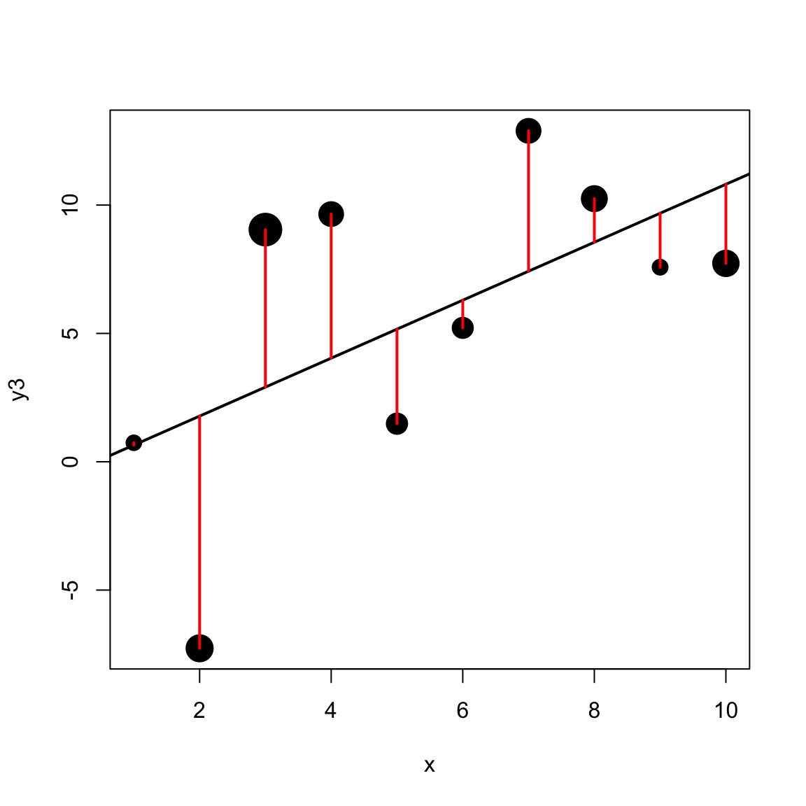
Different precision for different data points

Weighted Least Squares

Minimize Weighted \(SS_{residuals} = W_i\sum(Y_{i} - \widehat{Y})^2\)

Why weight?

Minimized influence of heteroskedasticity
Increases precision of estimates
Decreases influence of imprecision in measurements
Minimize sampling bias
Other reasons to count some measurements more than others

Weighted Least Squares

\[Y_i = \beta X_i + \epsilon_i\] \[\epsilon_i \sim \mathcal{N}(0, \sigma_i)\]
OLS: \(\sigma_1 = \sigma_2 = ...\) is constant
WLS: \(\sigma_i\) is variable

Generalized Least Squares

\[Y_i = \beta X_i + \epsilon_i\] \[\epsilon_i \sim \mathcal{N}(0, \sigma_i)\]
In OLS, this implies \(\sigma_i = \sigma I_n\)
(\(I_n\) is an identity matrix with n x n dimensions)

In WLS, the diagonal of the \(\sigma\) matrix can be anything

In Generalized Least Squares, the off diagonals can be non-zero, too

How can we use weighting?

Weighting by variance
Mean-Variance relationship
Unequal variance between groups

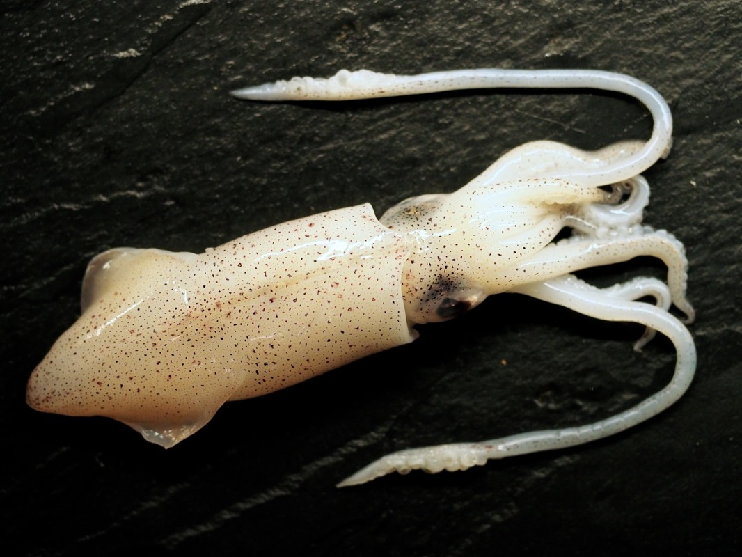
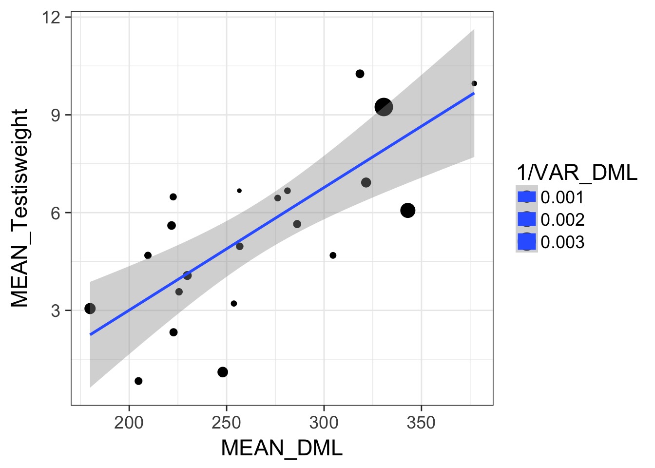
SQUID!

Somatic v. Reproductive Tissues: Variance

Somatic v. Reproductive Tissues: N

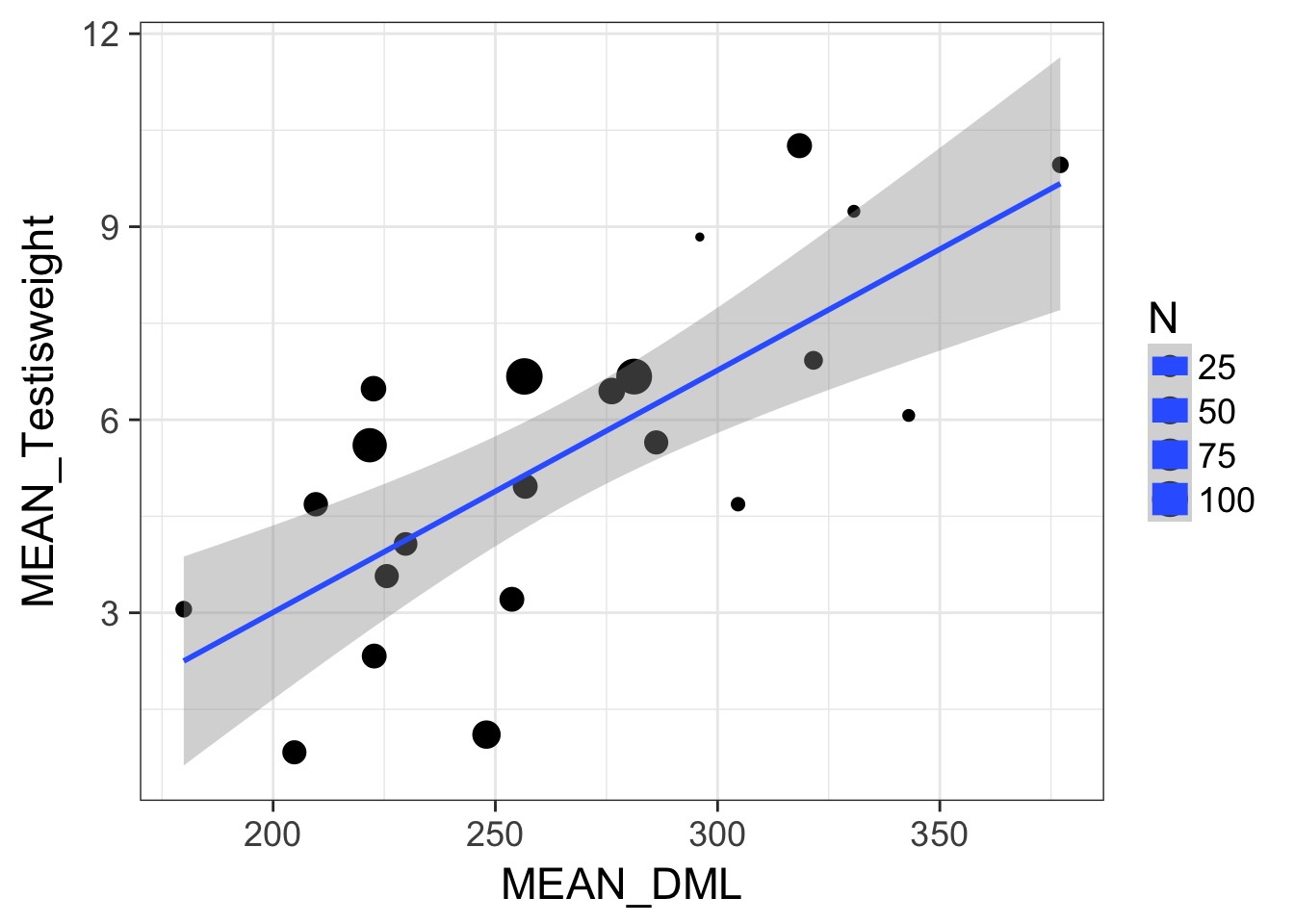
Weighting by Data Quality

We typically weight by 1/variance (precision)
- Or N, or other estimate of sample precision
This is different than variance weighted meta-analysis
- We are still estimating a residual error for fits

Implementation

sq_sum <- lm(MEAN_Testisweight ~ MEAN_DML, data=squid_summary,
             weights=1/VAR_DML)

Did it do anything?

No weights

term	estimate	std.error	statistic	p.value
(Intercept)	-4.5177727	2.1081505	-2.143003	0.0445948
MEAN_DML	0.0376229	0.0077701	4.842035	0.0000989

Precision Weighted

term	estimate	std.error	statistic	p.value
(Intercept)	-4.518775	2.2041869	-2.050087	0.0544130
MEAN_DML	0.037140	0.0074578	4.980010	0.0000831

Sample Size Weighted

term	estimate	std.error	statistic	p.value
(Intercept)	-5.2808150	2.8213670	-1.871722	0.0759446
MEAN_DML	0.0417104	0.0110373	3.779050	0.0011787

How can we use weighting?

Weighting by variance
Mean-Variance relationship
Unequal variance between groups

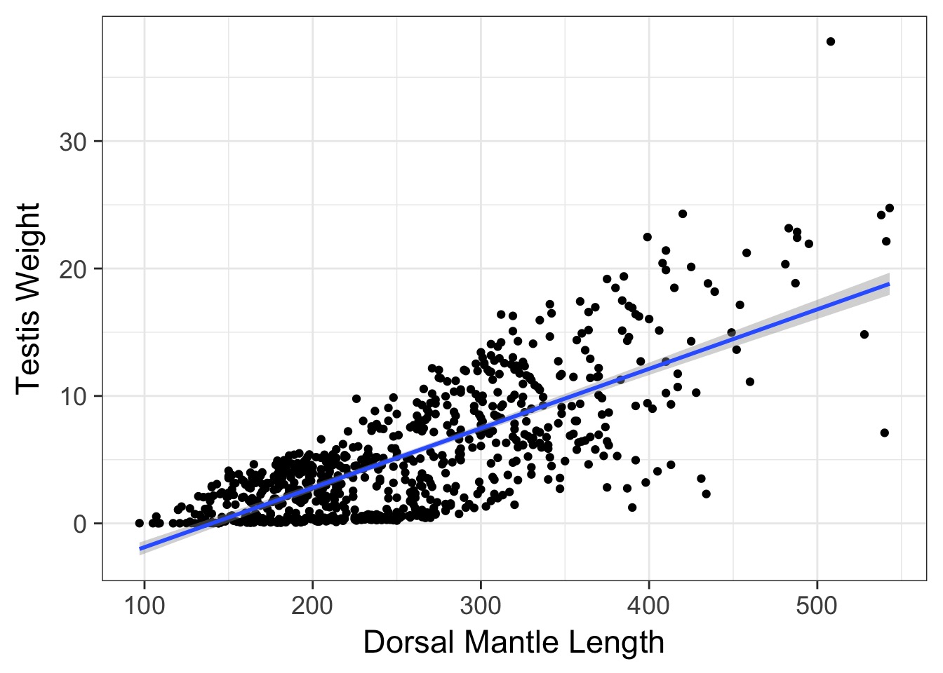
Looking at Individual Squid

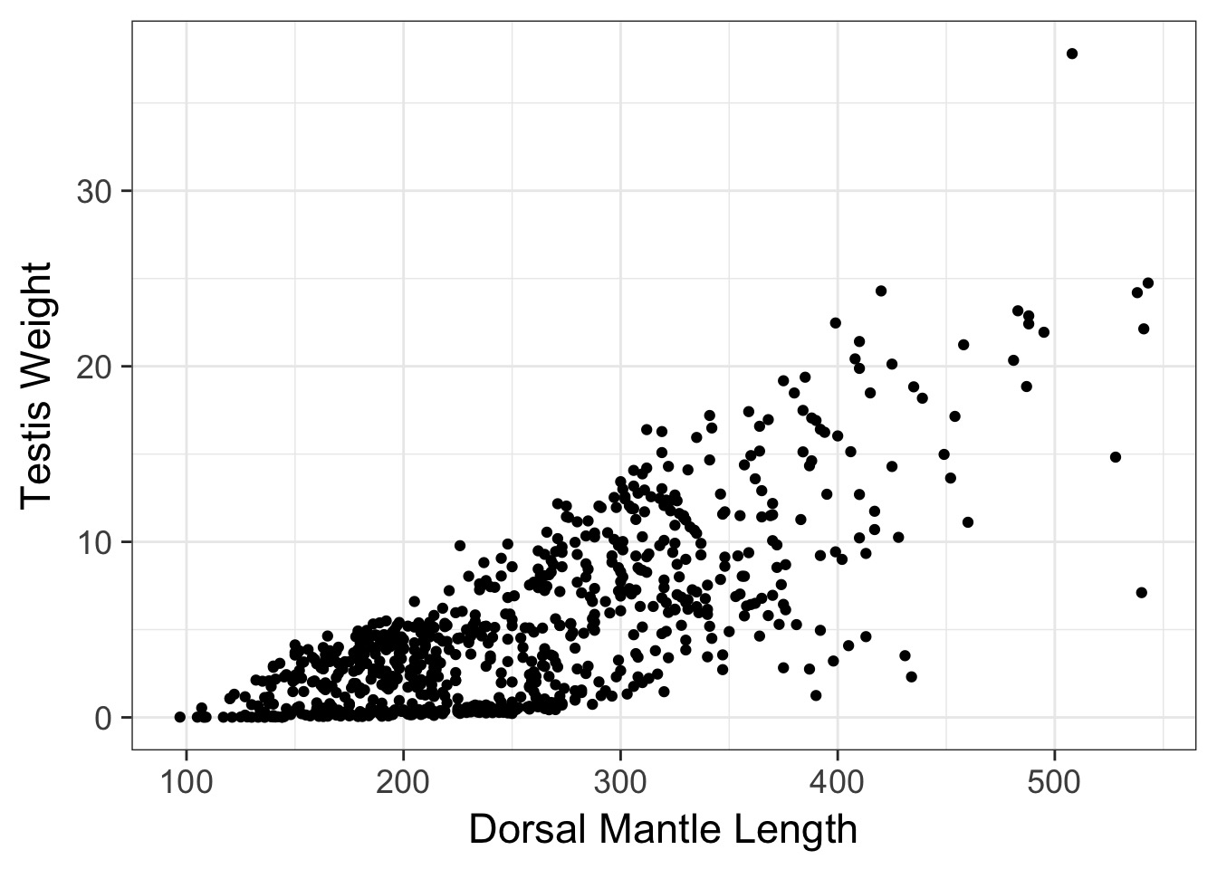
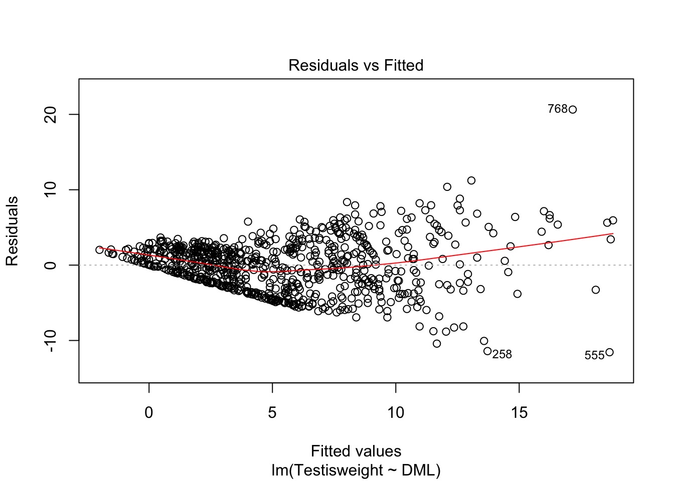
Oh, Yeah, That’s Heteroskedasticity

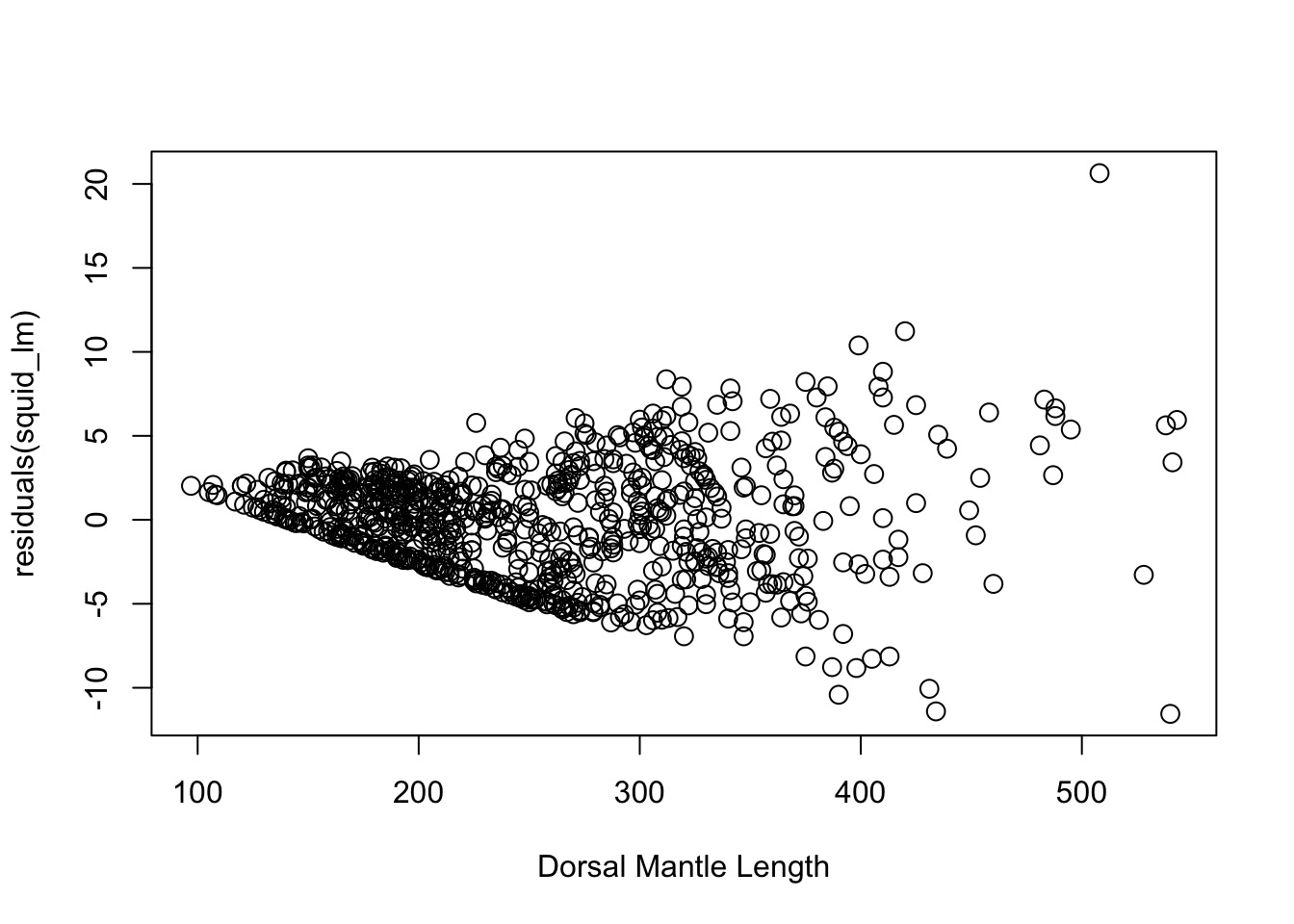
OK, But, We Need a test

Not every case is clear-cut
Breusch-Pagan/Godfrey/Koenker test
- Variant of White’s test (you’ll see this)
- Get squared residuals
- Regress on one or more predictors
- Results fail \(\chi^2\) test of heteroskedastic

BP Test

library(lmtest)

squid_lm <- lm(Testisweight ~ DML, data=squid)

bptest(squid_lm)


    studentized Breusch-Pagan test

data:  squid_lm
BP = 155.31, df = 1, p-value < 2.2e-16

Can use BP to Look at Multiple Predictors

squid_lm2 <- lm(Testisweight ~ DML + MONTH, data=squid)

bptest(squid_lm2)


    studentized Breusch-Pagan test

data:  squid_lm2
BP = 144.22, df = 2, p-value < 2.2e-16

Can Look at Contribution of Individual Predictors

bptest(squid_lm2, varformula = ~ DML, data=squid)


    studentized Breusch-Pagan test

data:  squid_lm2
BP = 140.74, df = 1, p-value < 2.2e-16

bptest(squid_lm2, varformula = ~ MONTH, data=squid)


    studentized Breusch-Pagan test

data:  squid_lm2
BP = 0.086946, df = 1, p-value = 0.7681

So How do we Weight This?

Weighting by a Predictor

Need to determine the direction variance increases
Weight by X or 1/X
Is it a linear or nonlinear relationship between variance and X?
Is more than one predictor influencing variance (from BP Test/Graphs)

WLS with LM

squid_wls <- lm(Testisweight ~ DML, data=squid,
                weights = 1/squid$DML)

Variance increases with DML, so weight decreases

LM is LiMiting

Need to hand-code the weights
Diagnostic plots will still look odd
- DHARMa can help
Cannot easily combine weights from multiple predictors

Enter NLME

NonLinear Mixed Effects Model package
We’ll get to what that means
BUT - also has likelihood-based methods to fit WLS and GLS
Flexible weighting specification

WLS via GLS in NLME

squid_gls <- gls(Testisweight ~ DML, 
                 
                 data=squid,
                 
                 weights = varFixed(~ DML))

Note: higher value = higher variance - opposite of lm

Compare WLS and GLS

WLS with lm


t test of coefficients:

              Estimate Std. Error t value  Pr(>|t|)    
(Intercept) -5.6239370  0.3382932 -16.624 < 2.2e-16 ***
DML          0.0430654  0.0014061  30.627 < 2.2e-16 ***
---
Signif. codes:  0 '***' 0.001 '**' 0.01 '*' 0.05 '.' 0.1 ' ' 1

GLS with gls


z test of coefficients:

              Estimate Std. Error z value  Pr(>|z|)    
(Intercept) -5.6239370  0.3382932 -16.624 < 2.2e-16 ***
DML          0.0430654  0.0014061  30.627 < 2.2e-16 ***
---
Signif. codes:  0 '***' 0.001 '**' 0.01 '*' 0.05 '.' 0.1 ' ' 1

Different Variance Structures

VarFixed - Linear continuous variance
VarPower - Variance increases by a power
VarExp - Variance exponentiated
VarConstPower - Variance is constant + power
VarIdent - Variance differs by groups
VarComb - Combines different variance functions

Multiple Sources of Heteroskedasticity

Let’s add month! If it was another driver…

squid_gls_month <- gls(Testisweight ~ DML, data=squid,

                       weights = varComb(varFixed(~DML),
                                         
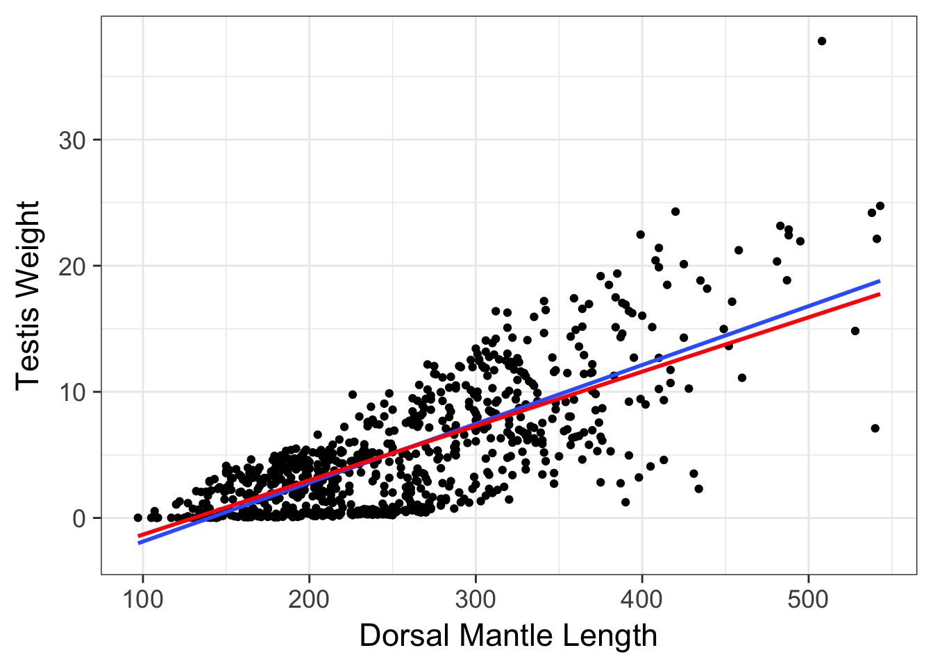
                                         varFixed(~MONTH)))

Weighted v. Naieve Fit

How can we use weighting?

Weighting by variance
Mean-Variance relationship
Unequal variance between groups

Testis Weight by Month

squid <- mutate(squid, fMONTH = factor(MONTH))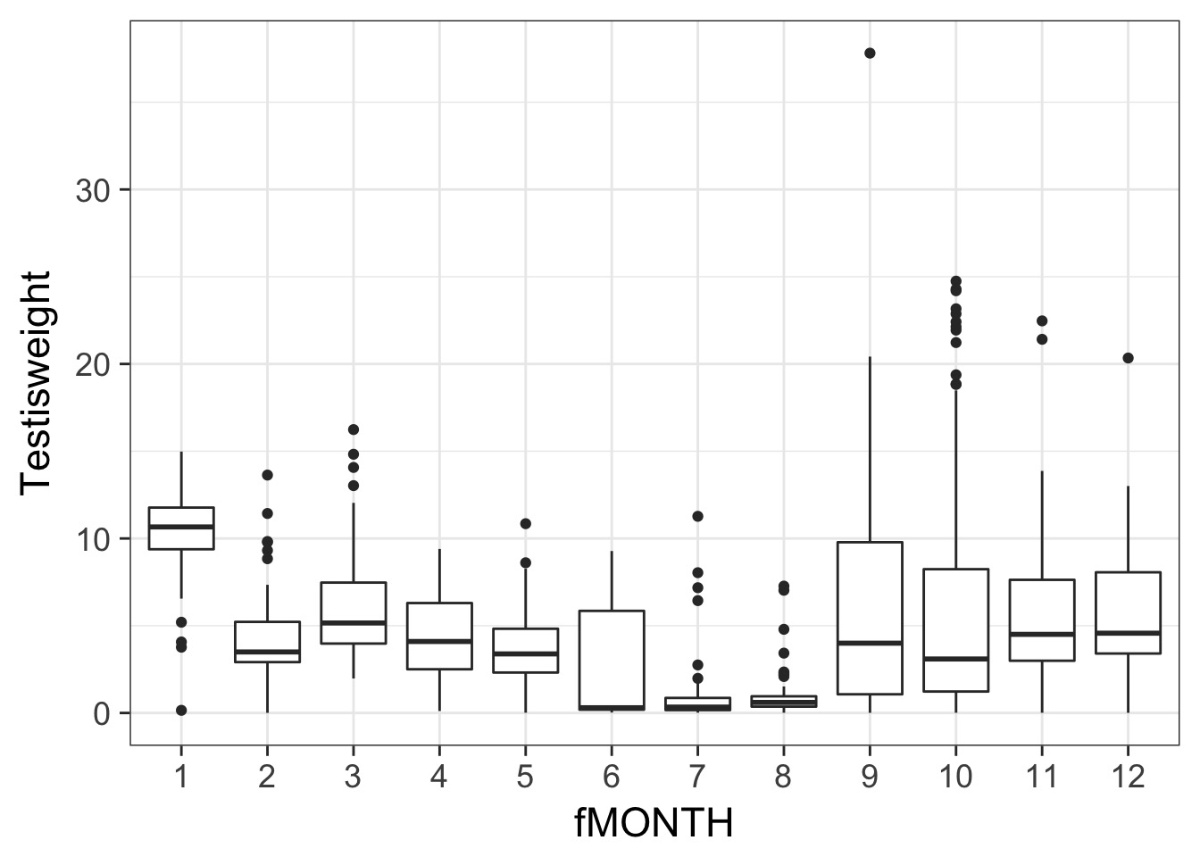

A Classic ANOVA problem

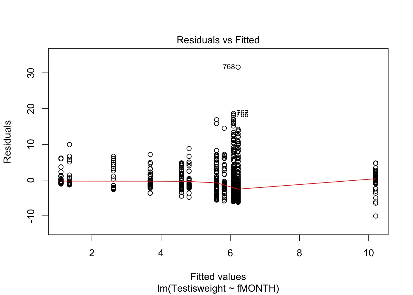
Wowsers - Unequal Variances

MONTH	var_weight
1	8.216093
2	9.491376
3	9.456260
4	6.663934
5	5.513464
6	10.884092
7	6.635753
8	2.274724
9	41.502657
10	46.016877
11	17.488115
12	17.734229

Is this a probem?

bptest(squid_month)


    studentized Breusch-Pagan test

data:  squid_month
BP = 68.375, df = 11, p-value = 2.485e-10

Solution: Weight by Month

vMonth <- varIdent(form = ~ 1 | fMONTH)

Note 1 | x form, different variance for different strata

Fit and Estimate SD

squid_month_gls <- gls(Testisweight ~ fMONTH, 
                       
                       data=squid, 
                       
                       weights=vMonth)

Summary of results

Generalized least squares fit by REML
  Model: Testisweight ~ fMONTH 
  Data: squid 
       AIC      BIC   logLik
  4307.961 4419.034 -2129.98

Variance function:
 Structure: Different standard deviations per stratum
 Formula: ~1 | fMONTH 
 Parameter estimates:
        2         9        12        11         8        10         5 
1.0000000 2.0910010 1.3669006 1.3573650 0.4895507 2.2018372 0.7621603 
        7         6         4         1         3 
0.8361282 1.0708259 0.8379144 0.9303731 0.9981328 

Coefficients:
                Value Std.Error    t-value p-value
(Intercept) 10.200311 0.4272917  23.872011       0
fMONTH2     -5.391282 0.6795202  -7.933953       0
fMONTH3     -4.094684 0.5555744  -7.370183       0
fMONTH4     -5.609615 0.5722338  -9.803013       0
fMONTH5     -6.514285 0.5724285 -11.380085       0
fMONTH6     -7.577601 0.6848334 -11.064882       0
fMONTH7     -8.847744 0.6016011 -14.706993       0
fMONTH8     -9.093561 0.4757355 -19.114743       0
fMONTH9     -3.975147 0.7016302  -5.665587       0
fMONTH10    -4.109998 0.7252503  -5.667006       0
fMONTH11    -4.596277 0.6174994  -7.443371       0
fMONTH12    -4.373843 0.7482711  -5.845265       0

 Correlation: 
         (Intr) fMONTH2 fMONTH3 fMONTH4 fMONTH5 fMONTH6 fMONTH7 fMONTH8
fMONTH2  -0.629                                                        
fMONTH3  -0.769  0.484                                                 
fMONTH4  -0.747  0.470   0.574                                         
fMONTH5  -0.746  0.469   0.574   0.557                                 
fMONTH6  -0.624  0.392   0.480   0.466   0.466                         
fMONTH7  -0.710  0.447   0.546   0.530   0.530   0.443                 
fMONTH8  -0.898  0.565   0.691   0.671   0.670   0.560   0.638         
fMONTH9  -0.609  0.383   0.468   0.455   0.455   0.380   0.433   0.547 
fMONTH10 -0.589  0.370   0.453   0.440   0.440   0.368   0.418   0.529 
fMONTH11 -0.692  0.435   0.532   0.517   0.517   0.432   0.491   0.622 
fMONTH12 -0.571  0.359   0.439   0.426   0.426   0.356   0.406   0.513 
         fMONTH9 fMONTH10 fMONTH11
fMONTH2                           
fMONTH3                           
fMONTH4                           
fMONTH5                           
fMONTH6                           
fMONTH7                           
fMONTH8                           
fMONTH9                           
fMONTH10  0.359                   
fMONTH11  0.421   0.408           
fMONTH12  0.348   0.336    0.395  

Standardized residuals:
       Min         Q1        Med         Q3        Max 
-3.5056004 -0.6728254 -0.3252821  0.4762647  4.9030307 

Residual standard error: 3.080871 
Degrees of freedom: 768 total; 756 residual

Compare with Unweighted Fit

squid_lm <- gls(Testisweight ~ fMONTH, data=squid)

anova(squid_lm, squid_month_gls)

                Model df      AIC      BIC    logLik   Test L.Ratio
squid_lm            1 13 4555.853 4616.017 -2264.926               
squid_month_gls     2 24 4307.961 4419.034 -2129.980 1 vs 2 269.892
                p-value
squid_lm               
squid_month_gls  <.0001

A Clammy Example

Clams.txt has data on the length-AFDM relationship of Wedge clames in Argentina each month.
- Use read.delim to read it in
Evaluate the length-biomass relationship
- Test for Heteroskedasticity
- Correct for it
Do the same for just month
- You’ll have to make it a factor
Combine them into one model!
- use varComb