Back to Bayes-ics

Bayesian Inference

• Frequentist: p(x ≤ D | H)
  
  
  
• Likelhoodist: p( D | H)
  
  
  
• Bayesian: p(H | D)

Why is this approach inherently Bayesian?

Let’s see how Bayes works

I have a bag with 4 stones. Some are black. Some are white.

I’m going to draw stones, one at a time, with replacement, and let’s see the number of ways that the draw could have been produced.

After 4 draws, let’s calculate the probability of W white stones and B black stones. Let’s formalize how we made this calculation - and derive Bayes Theorem!

Bayes Theorem and Stones

• Each possibility = H
  
  
• Prior plausibility = P(H)
  
  
• P(Draw | H) = Likelihood
  
  
• Sum of all P(Draw | H) P(H) = Average Likelihood
  - = P(Draw)

Bayes Theorem and Stones

\[p(H_i | Draw) = \frac{Likelihood\,* \,Prior}{Average\,\,Likelihood}\]

Bayes Theorem and Stones

\[p(H_i | Draw) = \frac{p(Draw | H_i) p(H_i)}{P(Draw)}\]

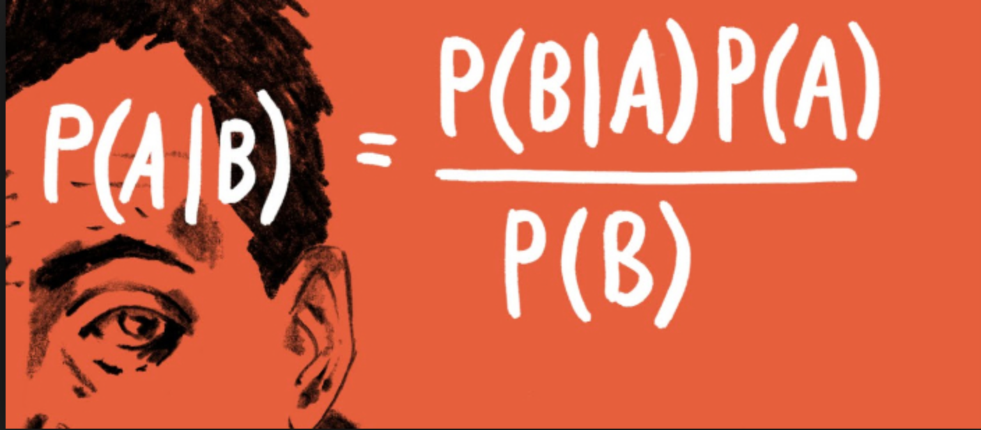
Bayes Theorem

\[p(Hypothesis | Data) = \frac{p(Data | Hypothesis) p(Hypothesis)}{P(Data)}\]

Bayesian Updating

Now let’s do that over again! And again!

Watch the Updating in Realtime!

Let’s do this in R with Grid Sampling!

Use dplyr and mutate() for the following.

0. Chose what fraction of stones is white in a bag of infinite size.
   
   
1. Creat a column of possible values from 0 to 1.
   
   
2. Define a prior as the second column.
   
   
3. Calculate your posterior after 1 random draw, then repeat for draws 2-4 plotting your posteriors
   • posterior = likelihood*prior/sum(all posterior values)
     
     
4. Plot your posterior given 100 draws, given your initial prior.

Introducing rethinking

library(rethinking)

#alist is a list for used to define a model
some_model <- alist(
  
  #our likelihood

  #our prior - can be something else if you want!
)

#define the data - you fill in the probability
some_data <- list(...)

#We will use map - maximum a posteriori sampling
#Note, I use rethinking:: in case you've loaded purrr
some_fit <- rethinking::map(some_model,
                             data = some_data)

Introducing rethinking

This is from the Rcode on page 42, box 2.6. Assume 100 draws.

library(rethinking)

#alist is a list for used to define a model
draws_mod <- alist(
  
  #our likelihood
  w ~ dbinom(100, p),
  
  #our prior - can be something else if you want!
  p ~ dunif(0,1)
)

#define the data - you fill in the number of successes
draws_data <- list(w = 32)

#We will use map - maximum a posteriori sampling
#Note, I use rethinking:: in case you've loaded purrr
draws_fit <- rethinking::map(draws_mod,
                             data = draws_data)

Now let’s explore our output

draws_fit

Maximum a posteriori (MAP) model fit

Formula:
w ~ dbinom(100, p)
p ~ dunif(0, 1)

MAP values:
        p 
0.3200005 

Log-likelihood: -2.46 

Summary

summary(draws_fit)

  Mean StdDev 5.5% 94.5%
p 0.32   0.05 0.25  0.39

precis

precis(draws_fit, prob = 0.6)

  Mean StdDev 20.0% 80.0%
p 0.32   0.05  0.28  0.36

Evaluation of a Posterior: Bayesian Credible Intervals

Evaluation of a Posterior: Frequentist Confidence Intervals

\[\hat{\beta} - t(\alpha, df)SE_{\beta} \le \beta \le \hat{\beta} +t(\alpha, df)SE_{\beta}\]

Credible Intervals versus Confidence Intervals

• Frequentist Confidence Intervals tell you the region you have confidence a true value of a parameter may occur
  
  
• If you have an estimate of 5 with a Frequentist CI of 2, you cannot say how likely it is that the parameter is 3, 4, 5, 6, or 7
  
  
• Bayesian Credible Intervals tell you the region that you have some probability of a parameter value
  
  
• With an estimate of 5 and a CI of 2, you can make statements about degree of belief in whether a parmeter is 3, 4,5, 6 or 7 - or even the probability that it falls outside of those bounds

The Posterior with extract.samples

draws_fit %>% extract.samples() %>%
  head()

          p
1 0.3544378
2 0.2834933
3 0.3437578
4 0.2504989
5 0.3051117
6 0.3089026

Visualize the posterior

Your turn

• Fit a binomial model using rethinking with - 19 successes - 50 trials
   
• Plot it
  
  
• If you can, with geom_ribbon(), highlight the 75% CI